Chapter 15 MI5000: Ordered exploitation results

Here we present the results for best performances found by each selection scheme replicate on the ordered exploitation diagnostic with configurations presented below. Best performance found refers to the largest average trait score found in a given population. Note that performance values fall between 0.0 and 100.0. For our the configuration of these experiments, we execute migrations every 50 generations and there are 4 islands in a ring topology. When migrations occur, we swap two individuals (same position on each island) and guarantee that no solution can return to the same island.

15.1 Analysis dependencies

library(ggplot2)
library(cowplot)
library(dplyr)
library(PupillometryR)

15.2 Truncation selection

Here we analyze how the different population structures affect truncation selection (size 8) on the ordered exploitation diagnostic.

15.2.1 Performance over time

lines = filter(mi5000_over_time, Diagnostic == 'ORDERED_EXPLOITATION' & `Selection\nScheme` == 'TRUNCATION') %>%
  group_by(Structure, Generations) %>%
  dplyr::summarise(
    min = min(pop_fit_max) / DIMENSIONALITY,
    mean = mean(pop_fit_max) / DIMENSIONALITY,
    max = max(pop_fit_max) / DIMENSIONALITY
  )
ggplot(lines, aes(x=Generations, y=mean, group = Structure, fill = Structure, color = Structure, shape = Structure)) +
  geom_ribbon(aes(ymin = min, ymax = max), alpha = 0.1) +
  geom_line(size = 0.5) +
  geom_point(data = filter(lines, Generations %% 2000 == 0), size = 2.5, stroke = 2.0, alpha = 1.0) +
  scale_y_continuous(
    name="Average trait score",
    limits=c(-1, 101),
    breaks=seq(0,100, 20),
    labels=c("0", "20", "40", "60", "80", "100")
  ) +
  scale_x_continuous(
    name="Generations",
    limits=c(0, 50000),
    breaks=c(0, 10000, 20000, 30000, 40000, 50000),
    labels=c("0e+4", "1e+4", "2e+4", "3e+4", "4e+4", "5e+4")

  ) +
  scale_shape_manual(values=SHAPE)+
  scale_colour_manual(values = cb_palette) +
  scale_fill_manual(values = cb_palette) +
  ggtitle("Performance over time") +
  p_theme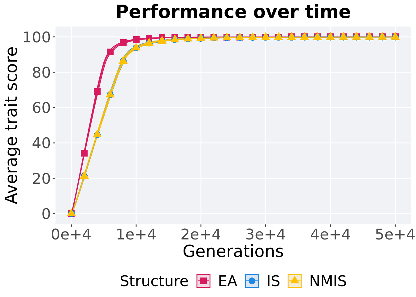

15.2.2 Generation satisfactory solution found

First generation a satisfactory solution is found throughout the 50,000 generations.

filter(mi5000_ssf, Diagnostic == 'ORDERED_EXPLOITATION' & `Selection\nScheme` == 'TRUNCATION') %>%
  ggplot(., aes(x = Structure, y = Generations , color = Structure, fill = Structure, shape = Structure)) +
  geom_flat_violin(position = position_nudge(x = .2, y = 0), scale = 'width', alpha = 0.2) +
  geom_point(position = position_jitter(width = .1), size = 1.5, alpha = 1.0) +
  geom_boxplot(color = 'black', width = .2, outlier.shape = NA, alpha = 0.0) +
  scale_y_continuous(
    name="Generation"
  ) +
  scale_x_discrete(
    name="Structure"
  )+
  scale_shape_manual(values=SHAPE)+
  scale_colour_manual(values = cb_palette, ) +
  scale_fill_manual(values = cb_palette) +
  ggtitle('Generation satisfactory solution found')+
  p_theme + coord_flip()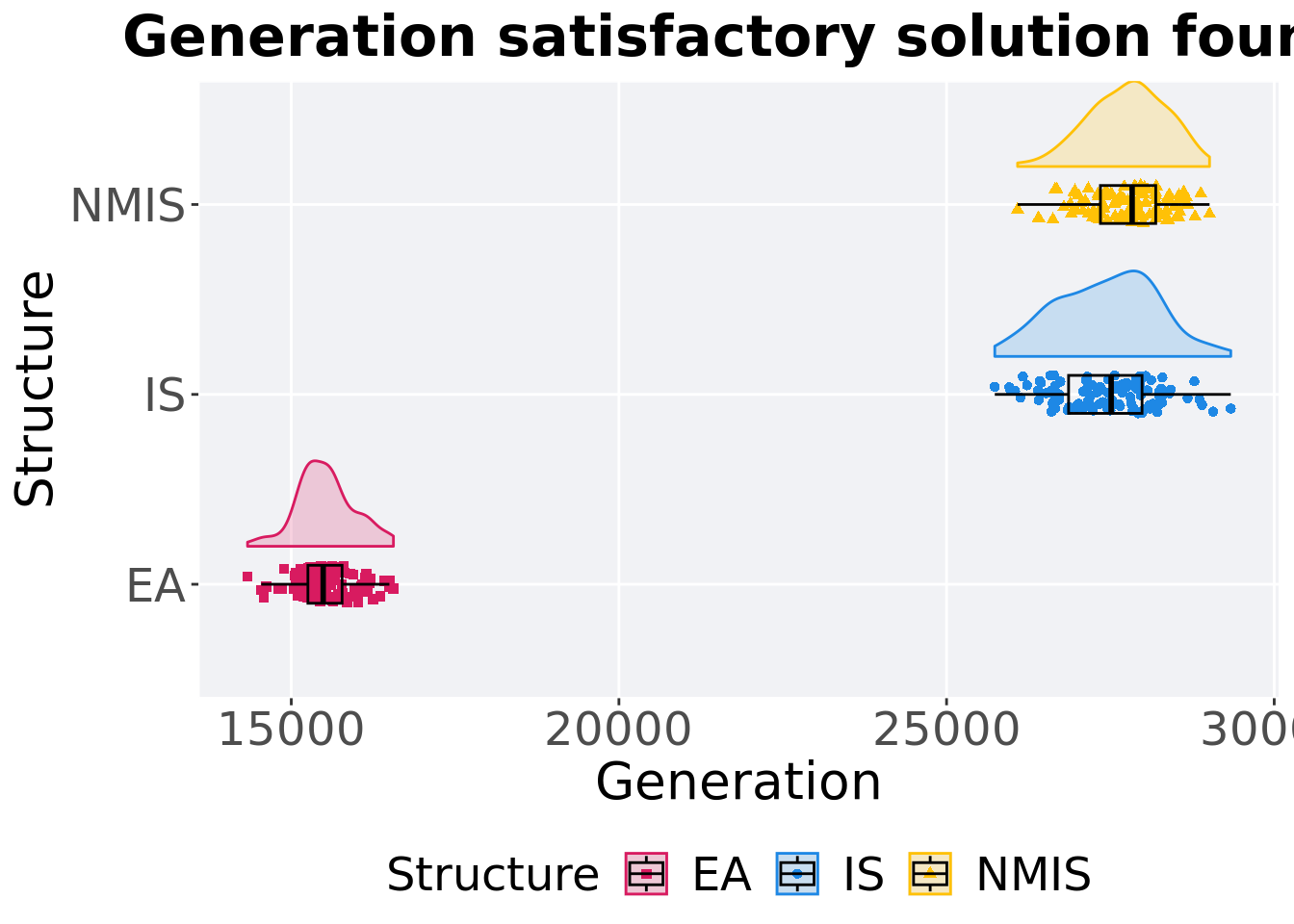

15.2.2.1 Stats

Summary statistics for the first generation a satisfactory solution is found.

ssf = filter(mi5000_ssf, Diagnostic == 'ORDERED_EXPLOITATION' & `Selection\nScheme` == 'TRUNCATION' & Generations < 60000)
ssf %>%
  group_by(Structure) %>%
  dplyr::summarise(
    count = n(),
    na_cnt = sum(is.na(Generations)),
    min = min(Generations, na.rm = TRUE),
    median = median(Generations, na.rm = TRUE),
    mean = mean(Generations, na.rm = TRUE),
    max = max(Generations, na.rm = TRUE),
    IQR = IQR(Generations, na.rm = TRUE)
  )

## # A tibble: 3 x 8
##   Structure count na_cnt   min median   mean   max   IQR
##   <fct>     <int>  <int> <int>  <dbl>  <dbl> <int> <dbl>
## 1 EA          100      0 14333 15487  15522. 16559  521.
## 2 IS          100      0 25736 27512. 27446. 29337 1121.
## 3 NMIS        100      0 26084 27832  27762. 29013  844.

Kruskal–Wallis test provides evidence of difference among selection schemes.

kruskal.test(Generations ~ Structure, data = ssf)

## 
##  Kruskal-Wallis rank sum test
## 
## data:  Generations by Structure
## Kruskal-Wallis chi-squared = 203.38, df = 2, p-value < 2.2e-16

Results for post-hoc Wilcoxon rank-sum test with a Bonferroni correction.

pairwise.wilcox.test(x = ssf$Generations, g = ssf$Structure, p.adjust.method = "bonferroni",
                     paired = FALSE, conf.int = FALSE, alternative = 'g')

## 
##  Pairwise comparisons using Wilcoxon rank sum test with continuity correction 
## 
## data:  ssf$Generations and ssf$Structure 
## 
##      EA     IS    
## IS   <2e-16 -     
## NMIS <2e-16 0.0039
## 
## P value adjustment method: bonferroni

15.3 Tournament selection

Here we analyze how the different population structures affect tournament selection (size 8) on the ordered exploitation diagnostic.

15.3.1 Performance over time

lines = filter(mi5000_over_time, Diagnostic == 'ORDERED_EXPLOITATION' & `Selection\nScheme` == 'TOURNAMENT') %>%
  group_by(Structure, Generations) %>%
  dplyr::summarise(
    min = min(pop_fit_max) / DIMENSIONALITY,
    mean = mean(pop_fit_max) / DIMENSIONALITY,
    max = max(pop_fit_max) / DIMENSIONALITY
  )
ggplot(lines, aes(x=Generations, y=mean, group = Structure, fill = Structure, color = Structure, shape = Structure)) +
  geom_ribbon(aes(ymin = min, ymax = max), alpha = 0.1) +
  geom_line(size = 0.5) +
  geom_point(data = filter(lines, Generations %% 2000 == 0), size = 2.5, stroke = 2.0, alpha = 1.0) +
  scale_y_continuous(
    name="Average trait score",
    limits=c(-1, 101),
    breaks=seq(0,100, 20),
    labels=c("0", "20", "40", "60", "80", "100")
  ) +
  scale_x_continuous(
    name="Generations",
    limits=c(0, 50000),
    breaks=c(0, 10000, 20000, 30000, 40000, 50000),
    labels=c("0e+4", "1e+4", "2e+4", "3e+4", "4e+4", "5e+4")

  ) +
  scale_shape_manual(values=SHAPE)+
  scale_colour_manual(values = cb_palette) +
  scale_fill_manual(values = cb_palette) +
  ggtitle("Performance over time") +
  p_theme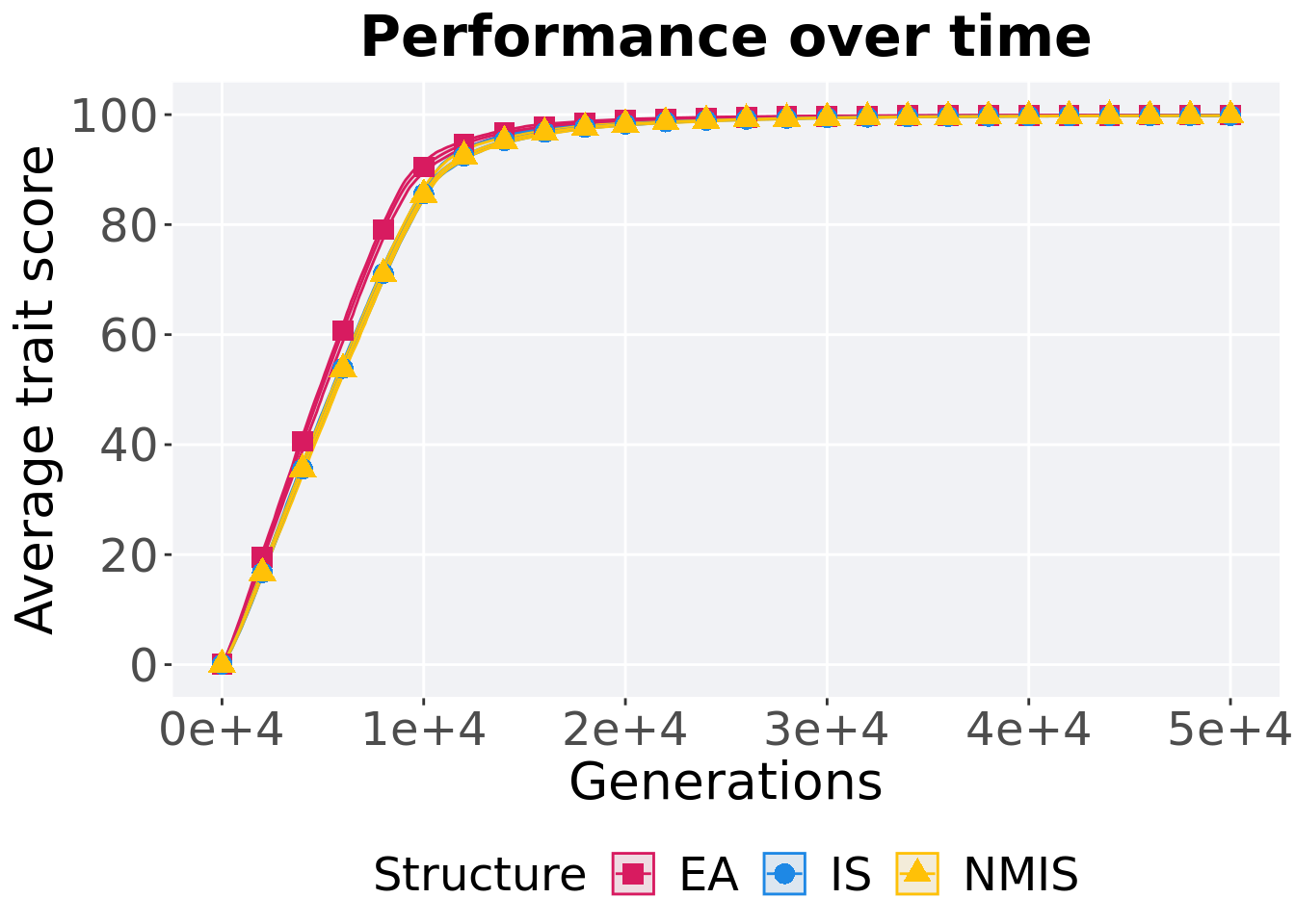

15.3.2 Generation satisfactory solution found

First generation a satisfactory solution is found throughout the 50,000 generations.

filter(mi5000_ssf, Diagnostic == 'ORDERED_EXPLOITATION' & `Selection\nScheme` == 'TOURNAMENT') %>%
  ggplot(., aes(x = Structure, y = Generations , color = Structure, fill = Structure, shape = Structure)) +
  geom_flat_violin(position = position_nudge(x = .2, y = 0), scale = 'width', alpha = 0.2) +
  geom_point(position = position_jitter(width = .1), size = 1.5, alpha = 1.0) +
  geom_boxplot(color = 'black', width = .2, outlier.shape = NA, alpha = 0.0) +
  scale_y_continuous(
    name="Generation"
  ) +
  scale_x_discrete(
    name="Structure"
  )+
  scale_shape_manual(values=SHAPE)+
  scale_colour_manual(values = cb_palette, ) +
  scale_fill_manual(values = cb_palette) +
  ggtitle('Generation satisfactory solution found')+
  p_theme + coord_flip()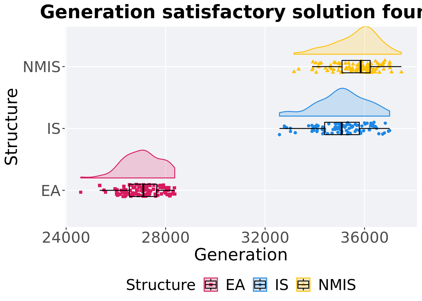

15.3.2.1 Stats

Summary statistics for the first generation a satisfactory solution is found.

ssf = filter(mi5000_ssf, Diagnostic == 'ORDERED_EXPLOITATION' & `Selection\nScheme` == 'TOURNAMENT' & Generations < 60000)
ssf %>%
  group_by(Structure) %>%
  dplyr::summarise(
    count = n(),
    na_cnt = sum(is.na(Generations)),
    min = min(Generations, na.rm = TRUE),
    median = median(Generations, na.rm = TRUE),
    mean = mean(Generations, na.rm = TRUE),
    max = max(Generations, na.rm = TRUE),
    IQR = IQR(Generations, na.rm = TRUE)
  )

## # A tibble: 3 x 8
##   Structure count na_cnt   min median   mean   max   IQR
##   <fct>     <int>  <int> <int>  <dbl>  <dbl> <int> <dbl>
## 1 EA          100      0 24586 27104. 27057. 28367 1101.
## 2 IS          100      0 32578 35082  35088. 37009 1392 
## 3 NMIS        100      0 33162 35845  35659. 37481 1130.

Kruskal–Wallis test provides evidence of difference among selection schemes.

kruskal.test(Generations ~ Structure, data = ssf)

## 
##  Kruskal-Wallis rank sum test
## 
## data:  Generations by Structure
## Kruskal-Wallis chi-squared = 206.91, df = 2, p-value < 2.2e-16

Results for post-hoc Wilcoxon rank-sum test with a Bonferroni correction.

pairwise.wilcox.test(x = ssf$Generations, g = ssf$Structure, p.adjust.method = "bonferroni",
                     paired = FALSE, conf.int = FALSE, alternative = 'g')

## 
##  Pairwise comparisons using Wilcoxon rank sum test with continuity correction 
## 
## data:  ssf$Generations and ssf$Structure 
## 
##      EA      IS     
## IS   < 2e-16 -      
## NMIS < 2e-16 5.6e-05
## 
## P value adjustment method: bonferroni

15.4 Lexicase selection

Here we analyze how the different population structures affect standard lexicase selection on the ordered exploitation diagnostic.

15.4.1 Performance over time

lines = filter(mi5000_over_time, Diagnostic == 'ORDERED_EXPLOITATION' & `Selection\nScheme` == 'LEXICASE') %>%
  group_by(Structure, Generations) %>%
  dplyr::summarise(
    min = min(pop_fit_max) / DIMENSIONALITY,
    mean = mean(pop_fit_max) / DIMENSIONALITY,
    max = max(pop_fit_max) / DIMENSIONALITY
  )
ggplot(lines, aes(x=Generations, y=mean, group = Structure, fill = Structure, color = Structure, shape = Structure)) +
  geom_ribbon(aes(ymin = min, ymax = max), alpha = 0.1) +
  geom_line(size = 0.5) +
  geom_point(data = filter(lines, Generations %% 2000 == 0), size = 2.5, stroke = 2.0, alpha = 1.0) +
  scale_y_continuous(
    name="Average trait score",
    limits=c(-1, 101),
    breaks=seq(0,100, 20),
    labels=c("0", "20", "40", "60", "80", "100")
  ) +
  scale_x_continuous(
    name="Generations",
    limits=c(0, 50000),
    breaks=c(0, 10000, 20000, 30000, 40000, 50000),
    labels=c("0e+4", "1e+4", "2e+4", "3e+4", "4e+4", "5e+4")

  ) +
  scale_shape_manual(values=SHAPE)+
  scale_colour_manual(values = cb_palette) +
  scale_fill_manual(values = cb_palette) +
  ggtitle("Performance over time") +
  p_theme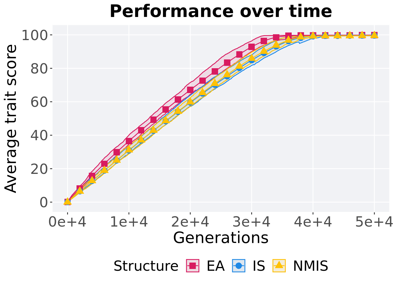

15.4.2 Best performance

First generation a satisfactory solution is found throughout the 50,000 generations.

filter(mi5000_best, Diagnostic == 'ORDERED_EXPLOITATION' & `Selection\nScheme` == 'LEXICASE' & VAR == 'pop_fit_max') %>%
  ggplot(., aes(x = Structure, y = VAL / DIMENSIONALITY, color = Structure, fill = Structure, shape = Structure)) +
  geom_flat_violin(position = position_nudge(x = .2, y = 0), scale = 'width', alpha = 0.2) +
  geom_point(position = position_jitter(width = .1), size = 1.5, alpha = 1.0) +
  geom_boxplot(color = 'black', width = .2, outlier.shape = NA, alpha = 0.0) +
  scale_y_continuous(
    name="Average trait score"
  ) +
  scale_x_discrete(
    name="Structure"
  )+
  scale_shape_manual(values=SHAPE)+
  scale_colour_manual(values = cb_palette, ) +
  scale_fill_manual(values = cb_palette) +
  ggtitle('Best performance')+
  p_theme + coord_flip()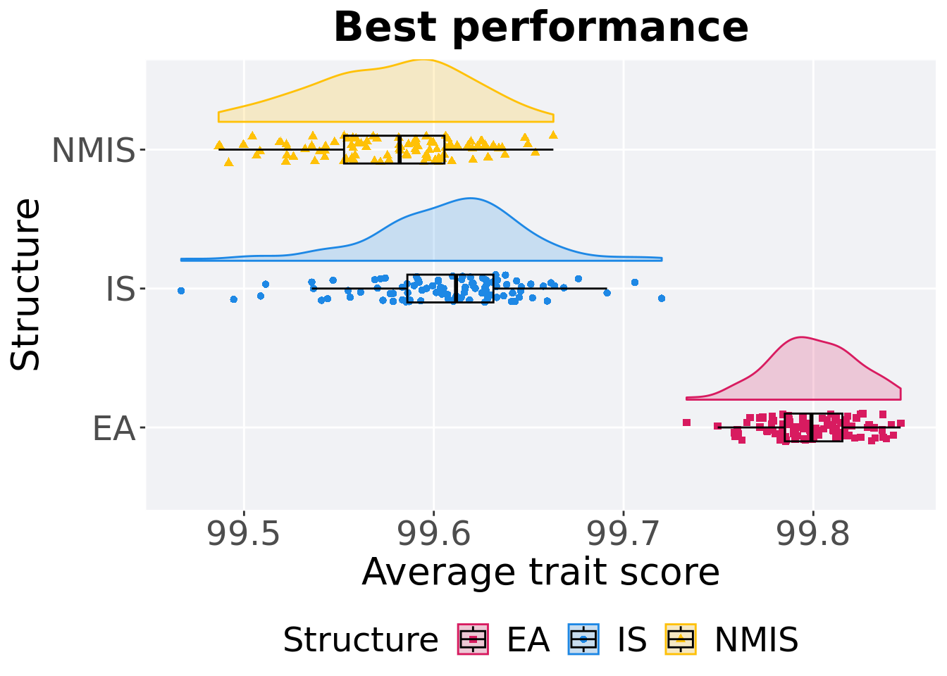

15.4.2.1 Stats

Summary statistics for the first generation a satisfactory solution is found.

performance = filter(mi5000_best, Diagnostic == 'ORDERED_EXPLOITATION' & `Selection\nScheme` == 'LEXICASE' & VAR == 'pop_fit_max')
performance %>%
  group_by(Structure) %>%
  dplyr::summarise(
    count = n(),
    na_cnt = sum(is.na(VAL)),
    min = min(VAL, na.rm = TRUE) / DIMENSIONALITY,
    median = median(VAL, na.rm = TRUE) / DIMENSIONALITY,
    mean = mean(VAL, na.rm = TRUE) / DIMENSIONALITY,
    max = max(VAL, na.rm = TRUE) / DIMENSIONALITY,
    IQR = IQR(VAL, na.rm = TRUE) / DIMENSIONALITY
  )

## # A tibble: 3 x 8
##   Structure count na_cnt   min median  mean   max    IQR
##   <fct>     <int>  <int> <dbl>  <dbl> <dbl> <dbl>  <dbl>
## 1 EA          100      0  99.7   99.8  99.8  99.8 0.0303
## 2 IS          100      0  99.5   99.6  99.6  99.7 0.0454
## 3 NMIS        100      0  99.5   99.6  99.6  99.7 0.0529

Kruskal–Wallis test provides evidence of difference among selection schemes.

kruskal.test(VAL ~ Structure, data = performance)

## 
##  Kruskal-Wallis rank sum test
## 
## data:  VAL by Structure
## Kruskal-Wallis chi-squared = 211.11, df = 2, p-value < 2.2e-16

Results for post-hoc Wilcoxon rank-sum test with a Bonferroni correction.

pairwise.wilcox.test(x = performance$VAL, g = performance$Structure, p.adjust.method = "bonferroni",
                     paired = FALSE, conf.int = FALSE, alternative = 'l')

## 
##  Pairwise comparisons using Wilcoxon rank sum test with continuity correction 
## 
## data:  performance$VAL and performance$Structure 
## 
##      EA      IS     
## IS   < 2e-16 -      
## NMIS < 2e-16 4.1e-07
## 
## P value adjustment method: bonferroni

15.4.3 Final performance

First generation a satisfactory solution is found throughout the 50,000 generations.

filter(mi5000_over_time, Diagnostic == 'ORDERED_EXPLOITATION' & `Selection\nScheme` == 'LEXICASE' & Generations == 50000) %>%
  ggplot(., aes(x = Structure, y = pop_fit_max / DIMENSIONALITY, color = Structure, fill = Structure, shape = Structure)) +
  geom_flat_violin(position = position_nudge(x = .2, y = 0), scale = 'width', alpha = 0.2) +
  geom_point(position = position_jitter(width = .1), size = 1.5, alpha = 1.0) +
  geom_boxplot(color = 'black', width = .2, outlier.shape = NA, alpha = 0.0) +
  scale_y_continuous(
    name="Average trait score"
  ) +
  scale_x_discrete(
    name="Structure"
  )+
  scale_shape_manual(values=SHAPE)+
  scale_colour_manual(values = cb_palette, ) +
  scale_fill_manual(values = cb_palette) +
  ggtitle('Final performance')+
  p_theme + coord_flip()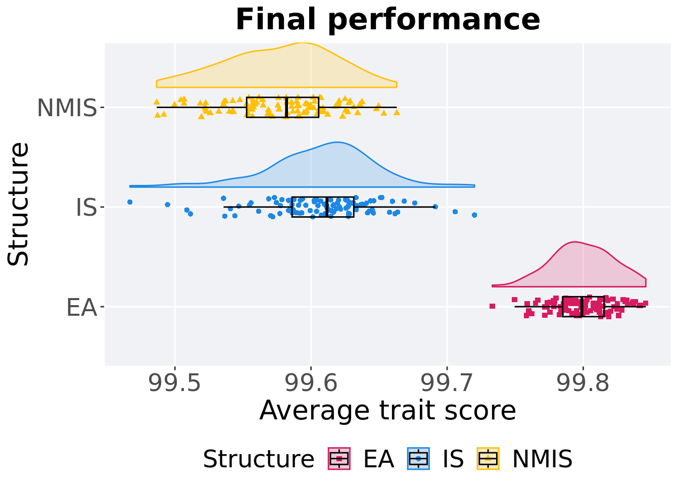

15.4.3.1 Stats

Summary statistics for the first generation a satisfactory solution is found.

performance = filter(mi5000_over_time, Diagnostic == 'ORDERED_EXPLOITATION' & `Selection\nScheme` == 'LEXICASE' & Generations == 50000)
performance %>%
  group_by(Structure) %>%
  dplyr::summarise(
    count = n(),
    na_cnt = sum(is.na(pop_fit_max)),
    min = min(pop_fit_max / DIMENSIONALITY, na.rm = TRUE),
    median = median(pop_fit_max / DIMENSIONALITY, na.rm = TRUE),
    mean = mean(pop_fit_max / DIMENSIONALITY, na.rm = TRUE),
    max = max(pop_fit_max / DIMENSIONALITY, na.rm = TRUE),
    IQR = IQR(pop_fit_max / DIMENSIONALITY, na.rm = TRUE)
  )

## # A tibble: 3 x 8
##   Structure count na_cnt   min median  mean   max    IQR
##   <fct>     <int>  <int> <dbl>  <dbl> <dbl> <dbl>  <dbl>
## 1 EA          100      0  99.7   99.8  99.8  99.8 0.0303
## 2 IS          100      0  99.5   99.6  99.6  99.7 0.0454
## 3 NMIS        100      0  99.5   99.6  99.6  99.7 0.0529

Kruskal–Wallis test provides evidence of difference among selection schemes.

kruskal.test(pop_fit_max ~ Structure, data = performance)

## 
##  Kruskal-Wallis rank sum test
## 
## data:  pop_fit_max by Structure
## Kruskal-Wallis chi-squared = 211.12, df = 2, p-value < 2.2e-16

Results for post-hoc Wilcoxon rank-sum test with a Bonferroni correction.

pairwise.wilcox.test(x = performance$pop_fit_max, g = performance$Structure, p.adjust.method = "bonferroni",
                     paired = FALSE, conf.int = FALSE, alternative = 'l')

## 
##  Pairwise comparisons using Wilcoxon rank sum test with continuity correction 
## 
## data:  performance$pop_fit_max and performance$Structure 
## 
##      EA     IS   
## IS   <2e-16 -    
## NMIS <2e-16 4e-07
## 
## P value adjustment method: bonferroni

15.4.4 Generation satisfactory solution found

First generation a satisfactory solution is found throughout the 50,000 generations.

lex_fail = filter(mi5000_ssf, Diagnostic == 'ORDERED_EXPLOITATION' & `Selection\nScheme` == 'LEXICASE' & GENERATIONS < Generations)
lex_fail$Generations = 55000
lex_fail$Structure <- factor(lex_fail$Structure, levels = MODEL)

filter(mi5000_ssf, Diagnostic == 'ORDERED_EXPLOITATION' & `Selection\nScheme` == 'LEXICASE'& Generations <= GENERATIONS) %>%
  ggplot(., aes(x = Structure, y = Generations, color = Structure, fill = Structure, shape = Structure)) +
    geom_flat_violin(position = position_nudge(x = .2, y = 0), scale = 'width', alpha = 0.2) +
  geom_point(position = position_jitter(width = .1), size = 1.5, alpha = 1.0) +
  geom_boxplot(color = 'black', width = .2, outlier.shape = NA, alpha = 0.0) +
  geom_point(data = lex_fail, aes(x = Structure, y = Generations, color = Structure, fill = Structure, shape = Structure),position = position_jitter(width = .05), size = 2.5) +
  scale_shape_manual(values=SHAPE)+
  scale_y_continuous(
    name="Generations",
    limits=c(30000, 55000),
    breaks=c(30000, 40000, 50000, 55000),
    labels=c("3e+4", "4e+4", "5e+4", "Fail")
  ) +
  scale_x_discrete(
    name="Structure"
  ) +
  scale_colour_manual(values = cb_palette) +
  scale_fill_manual(values = cb_palette) +
  p_theme + coord_flip()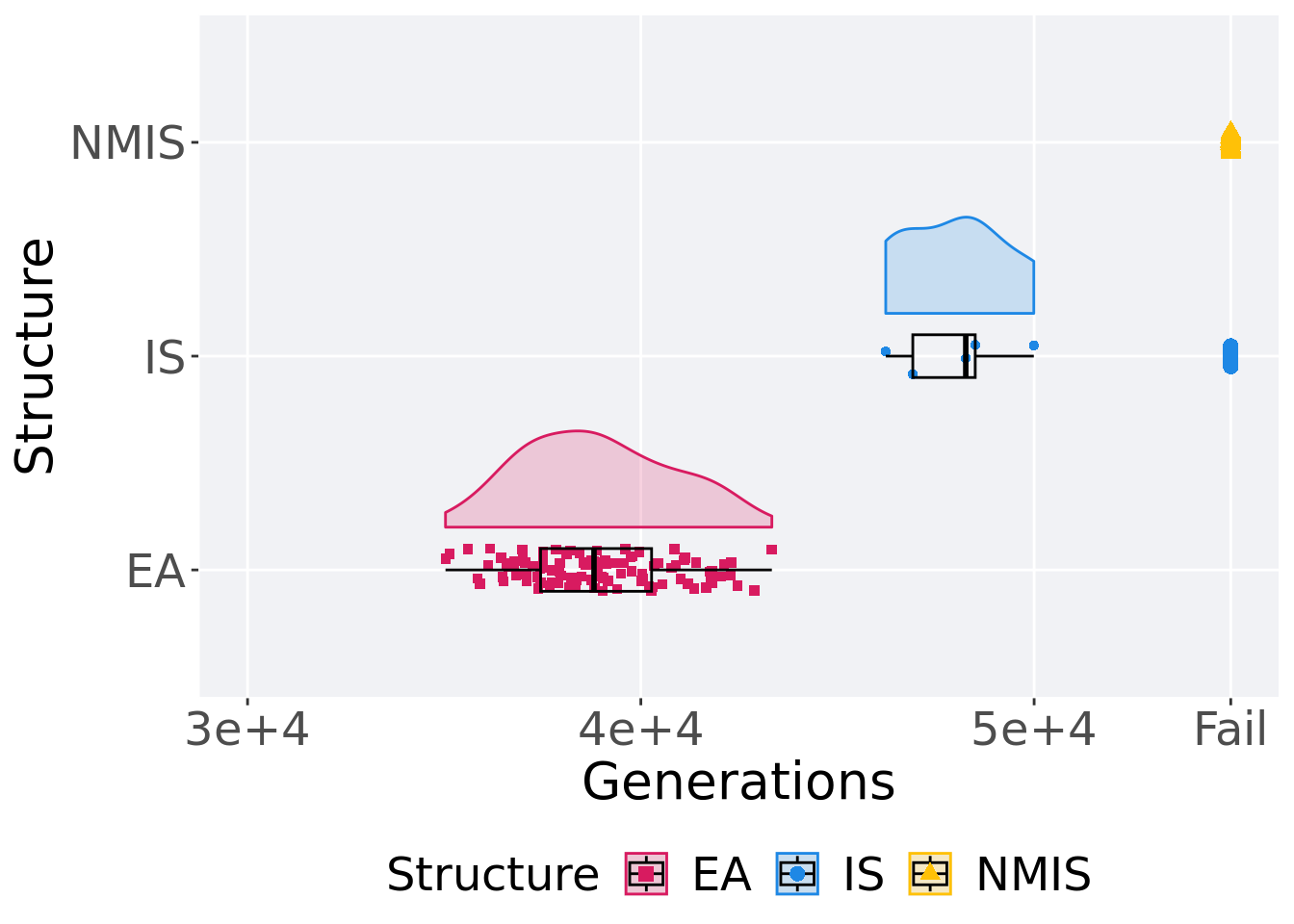

15.4.4.1 Stats

Summary statistics for the first generation a satisfactory solution is found.

ssf = filter(mi5000_ssf, Diagnostic == 'ORDERED_EXPLOITATION' & `Selection\nScheme` == 'LEXICASE' & Generations < 60000)
ssf %>%
  group_by(Structure) %>%
  dplyr::summarise(
    count = n(),
    na_cnt = sum(is.na(Generations)),
    min = min(Generations, na.rm = TRUE),
    median = median(Generations, na.rm = TRUE),
    mean = mean(Generations, na.rm = TRUE),
    max = max(Generations, na.rm = TRUE),
    IQR = IQR(Generations, na.rm = TRUE)
  )

## # A tibble: 2 x 8
##   Structure count na_cnt   min median   mean   max   IQR
##   <fct>     <int>  <int> <int>  <dbl>  <dbl> <int> <dbl>
## 1 EA          100      0 35033  38809 38906. 43331 2822.
## 2 IS            5      0 46227  48262 47980. 49992 1587

Kruskal–Wallis test provides evidence of difference among selection schemes.

kruskal.test(Generations ~ Structure, data = ssf)

## 
##  Kruskal-Wallis rank sum test
## 
## data:  Generations by Structure
## Kruskal-Wallis chi-squared = 14.151, df = 1, p-value = 0.0001687

Results for post-hoc Wilcoxon rank-sum test with a Bonferroni correction.

pairwise.wilcox.test(x = ssf$Generations, g = ssf$Structure, p.adjust.method = "bonferroni",
                     paired = FALSE, conf.int = FALSE, alternative = 'g')

## 
##  Pairwise comparisons using Wilcoxon rank sum test with continuity correction 
## 
## data:  ssf$Generations and ssf$Structure 
## 
##    EA     
## IS 8.7e-05
## 
## P value adjustment method: bonferroni