Chapter 10 MI50: Exploitation rate results

Here we present the results for best performances found by each selection scheme replicate on the exploitation rate diagnostic with configurations presented below. For our the configuration of these experiments, we execute migrations every 50 generations and there are 4 islands in a ring topology. When migrations occur, we swap two individuals (same position on each island) and guarantee that no solution can return to the same island. Best performance found refers to the largest average trait score found in a given population. Note that performance values fall between 0.0 and 100.0.

10.1 Analysis dependencies

library(ggplot2)
library(cowplot)
library(dplyr)
library(PupillometryR)

10.2 Truncation selection

Here we analyze how the different population structures affect truncation selection (size 8) on the exploitation rate diagnostic.

10.2.1 Performance over time

lines = filter(mi50_over_time, Diagnostic == 'EXPLOITATION_RATE' & `Selection\nScheme` == 'TRUNCATION') %>%
  group_by(Structure, Generations) %>%
  dplyr::summarise(
    min = min(pop_fit_max) / DIMENSIONALITY,
    mean = mean(pop_fit_max) / DIMENSIONALITY,
    max = max(pop_fit_max) / DIMENSIONALITY
  )
ggplot(lines, aes(x=Generations, y=mean, group = Structure, fill = Structure, color = Structure, shape = Structure)) +
  geom_ribbon(aes(ymin = min, ymax = max), alpha = 0.1) +
  geom_line(size = 0.5) +
  geom_point(data = filter(lines, Generations %% 2000 == 0), size = 2.5, stroke = 2.0, alpha = 1.0) +
  scale_y_continuous(
    name="Average trait score",
    limits=c(-1, 101),
    breaks=seq(0,100, 20),
    labels=c("0", "20", "40", "60", "80", "100")
  ) +
  scale_x_continuous(
    name="Generations",
    limits=c(0, 50000),
    breaks=c(0, 10000, 20000, 30000, 40000, 50000),
    labels=c("0e+4", "1e+4", "2e+4", "3e+4", "4e+4", "5e+4")

  ) +
  scale_shape_manual(values=SHAPE)+
  scale_colour_manual(values = cb_palette) +
  scale_fill_manual(values = cb_palette) +
  ggtitle("Best performance over time") +
  p_theme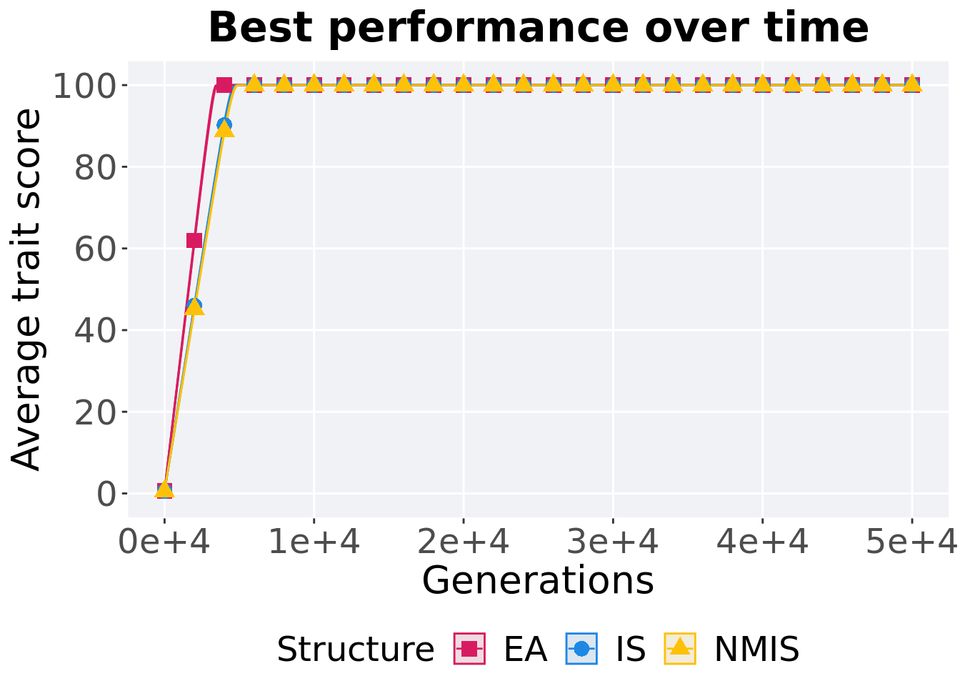

10.2.2 Generation satisfactory solution found

First generation a satisfactory solution is found throughout the 50,000 generations.

filter(mi50_ssf, Diagnostic == 'EXPLOITATION_RATE' & `Selection\nScheme` == 'TRUNCATION') %>%
  ggplot(., aes(x = Structure, y = Generations , color = Structure, fill = Structure, shape = Structure)) +
  geom_flat_violin(position = position_nudge(x = .2, y = 0), scale = 'width', alpha = 0.2) +
  geom_point(position = position_jitter(width = .1), size = 1.5, alpha = 1.0) +
  geom_boxplot(color = 'black', width = .2, outlier.shape = NA, alpha = 0.0) +
  scale_y_continuous(
    name="Generation"
  ) +
  scale_x_discrete(
    name="Structure"
  )+
  scale_shape_manual(values=SHAPE)+
  scale_colour_manual(values = cb_palette, ) +
  scale_fill_manual(values = cb_palette) +
  ggtitle('Generation satisfactory solution found')+
  p_theme + coord_flip()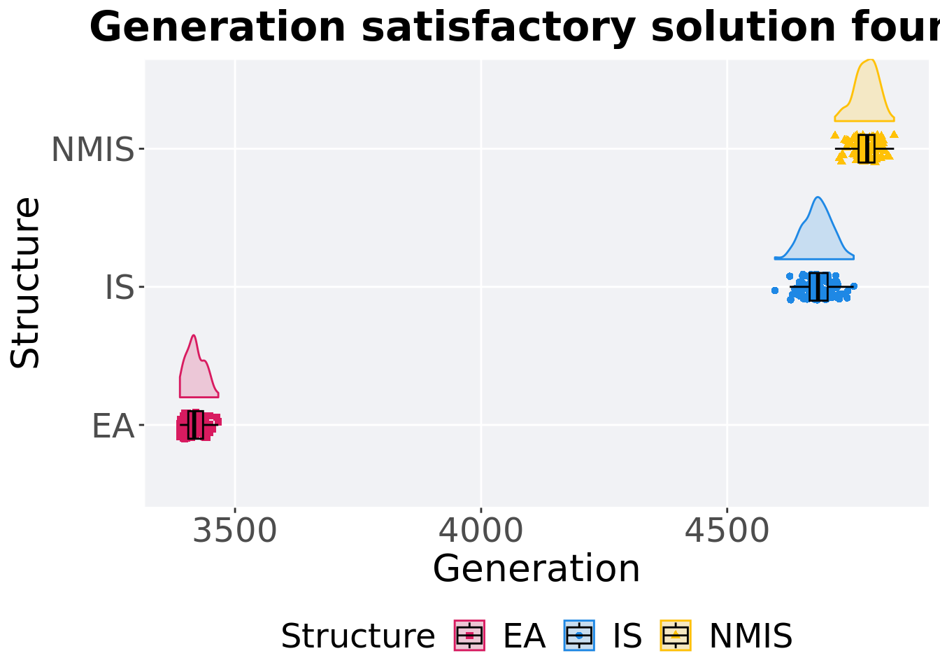

10.2.3 Stats

Summary statistics for the first generation a satisfactory solution is found.

ssf = filter(mi50_ssf, Diagnostic == 'EXPLOITATION_RATE' & `Selection\nScheme` == 'TRUNCATION' & Generations < 60000)
ssf %>%
  group_by(Structure) %>%
  dplyr::summarise(
    count = n(),
    na_cnt = sum(is.na(Generations)),
    min = min(Generations, na.rm = TRUE),
    median = median(Generations, na.rm = TRUE),
    mean = mean(Generations, na.rm = TRUE),
    max = max(Generations, na.rm = TRUE),
    IQR = IQR(Generations, na.rm = TRUE)
  )

## # A tibble: 3 x 8
##   Structure count na_cnt   min median  mean   max   IQR
##   <fct>     <int>  <int> <int>  <dbl> <dbl> <int> <dbl>
## 1 EA          100      0  3388  3417  3420.  3466  30  
## 2 IS          100      0  4597  4684. 4684.  4757  36.5
## 3 NMIS        100      0  4719  4784. 4783.  4839  32.2

Kruskal–Wallis test provides evidence of difference among selection schemes.

kruskal.test(Generations ~ Structure, data = ssf)

## 
##  Kruskal-Wallis rank sum test
## 
## data:  Generations by Structure
## Kruskal-Wallis chi-squared = 264.73, df = 2, p-value < 2.2e-16

Results for post-hoc Wilcoxon rank-sum test with a Bonferroni correction.

pairwise.wilcox.test(x = ssf$Generations, g = ssf$Structure, p.adjust.method = "bonferroni",
                     paired = FALSE, conf.int = FALSE, alternative = 'g')

## 
##  Pairwise comparisons using Wilcoxon rank sum test with continuity correction 
## 
## data:  ssf$Generations and ssf$Structure 
## 
##      EA     IS    
## IS   <2e-16 -     
## NMIS <2e-16 <2e-16
## 
## P value adjustment method: bonferroni

10.3 Tournament selection

Here we analyze how the different population structures affect tournament selection (size 8) on the exploitation rate diagnostic.

10.3.1 Performance over time

lines = filter(mi50_over_time, Diagnostic == 'EXPLOITATION_RATE' & `Selection\nScheme` == 'TOURNAMENT') %>%
  group_by(Structure, Generations) %>%
  dplyr::summarise(
    min = min(pop_fit_max) / DIMENSIONALITY,
    mean = mean(pop_fit_max) / DIMENSIONALITY,
    max = max(pop_fit_max) / DIMENSIONALITY
  )
ggplot(lines, aes(x=Generations, y=mean, group = Structure, fill = Structure, color = Structure, shape = Structure)) +
  geom_ribbon(aes(ymin = min, ymax = max), alpha = 0.1) +
  geom_line(size = 0.5) +
  geom_point(data = filter(lines, Generations %% 2000 == 0), size = 2.5, stroke = 2.0, alpha = 1.0) +
  scale_y_continuous(
    name="Average trait score",
    limits=c(-1, 101),
    breaks=seq(0,100, 20),
    labels=c("0", "20", "40", "60", "80", "100")
  ) +
  scale_x_continuous(
    name="Generations",
    limits=c(0, 50000),
    breaks=c(0, 10000, 20000, 30000, 40000, 50000),
    labels=c("0e+4", "1e+4", "2e+4", "3e+4", "4e+4", "5e+4")

  ) +
  scale_shape_manual(values=SHAPE)+
  scale_colour_manual(values = cb_palette) +
  scale_fill_manual(values = cb_palette) +
  ggtitle("Best performance over time") +
  p_theme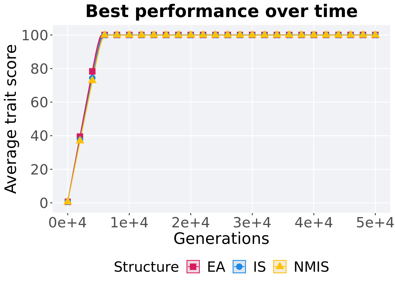

10.3.2 Generation satisfactory solution found

First generation a satisfactory solution is found throughout the 50,000 generations.

filter(mi50_ssf, Diagnostic == 'EXPLOITATION_RATE' & `Selection\nScheme` == 'TOURNAMENT') %>%
  ggplot(., aes(x = Structure, y = Generations , color = Structure, fill = Structure, shape = Structure)) +
  geom_flat_violin(position = position_nudge(x = .2, y = 0), scale = 'width', alpha = 0.2) +
  geom_point(position = position_jitter(width = .1), size = 1.5, alpha = 1.0) +
  geom_boxplot(color = 'black', width = .2, outlier.shape = NA, alpha = 0.0) +
  scale_y_continuous(
    name="Generation"
  ) +
  scale_x_discrete(
    name="Structure"
  )+
  scale_shape_manual(values=SHAPE)+
  scale_colour_manual(values = cb_palette, ) +
  scale_fill_manual(values = cb_palette) +
  ggtitle('Generation satisfactory solution found')+
  p_theme + coord_flip()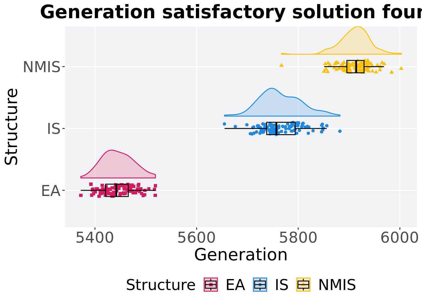

10.3.3 Stats

Summary statistics for the first generation a satisfactory solution is found.

ssf = filter(mi50_ssf, Diagnostic == 'EXPLOITATION_RATE' & `Selection\nScheme` == 'TOURNAMENT' & Generations < 60000)
ssf %>%
  group_by(Structure) %>%
  dplyr::summarise(
    count = n(),
    na_cnt = sum(is.na(Generations)),
    min = min(Generations, na.rm = TRUE),
    median = median(Generations, na.rm = TRUE),
    mean = mean(Generations, na.rm = TRUE),
    max = max(Generations, na.rm = TRUE),
    IQR = IQR(Generations, na.rm = TRUE)
  )

## # A tibble: 3 x 8
##   Structure count na_cnt   min median  mean   max   IQR
##   <fct>     <int>  <int> <int>  <dbl> <dbl> <int> <dbl>
## 1 EA          100      0  5372   5442 5446.  5519  44.5
## 2 IS          100      0  5655   5757 5765.  5882  56  
## 3 NMIS        100      0  5767   5914 5912.  6003  33.8

Kruskal–Wallis test provides evidence of difference among selection schemes.

kruskal.test(Generations ~ Structure, data = ssf)

## 
##  Kruskal-Wallis rank sum test
## 
## data:  Generations by Structure
## Kruskal-Wallis chi-squared = 264.22, df = 2, p-value < 2.2e-16

Results for post-hoc Wilcoxon rank-sum test with a Bonferroni correction.

pairwise.wilcox.test(x = ssf$Generations, g = ssf$Structure, p.adjust.method = "bonferroni",
                     paired = FALSE, conf.int = FALSE, alternative = 'g')

## 
##  Pairwise comparisons using Wilcoxon rank sum test with continuity correction 
## 
## data:  ssf$Generations and ssf$Structure 
## 
##      EA     IS    
## IS   <2e-16 -     
## NMIS <2e-16 <2e-16
## 
## P value adjustment method: bonferroni

10.4 Lexicase selection

Here we analyze how the different population structures affect standard lexicase selection on the exploitation rate diagnostic.

10.4.1 Performance over time

lines = filter(mi50_over_time, Diagnostic == 'EXPLOITATION_RATE' & `Selection\nScheme` == 'LEXICASE') %>%
  group_by(Structure, Generations) %>%
  dplyr::summarise(
    min = min(pop_fit_max) / DIMENSIONALITY,
    mean = mean(pop_fit_max) / DIMENSIONALITY,
    max = max(pop_fit_max) / DIMENSIONALITY
  )
ggplot(lines, aes(x=Generations, y=mean, group = Structure, fill = Structure, color = Structure, shape = Structure)) +
  geom_ribbon(aes(ymin = min, ymax = max), alpha = 0.1) +
  geom_line(size = 0.5) +
  geom_point(data = filter(lines, Generations %% 2000 == 0), size = 2.5, stroke = 2.0, alpha = 1.0) +
  scale_y_continuous(
    name="Average trait score",
    limits=c(-1, 101),
    breaks=seq(0,100, 20),
    labels=c("0", "20", "40", "60", "80", "100")
  ) +
  scale_x_continuous(
    name="Generations",
    limits=c(0, 50000),
    breaks=c(0, 10000, 20000, 30000, 40000, 50000),
    labels=c("0e+4", "1e+4", "2e+4", "3e+4", "4e+4", "5e+4")

  ) +
  scale_shape_manual(values=SHAPE)+
  scale_colour_manual(values = cb_palette) +
  scale_fill_manual(values = cb_palette) +
  ggtitle("Best performance over time") +
  p_theme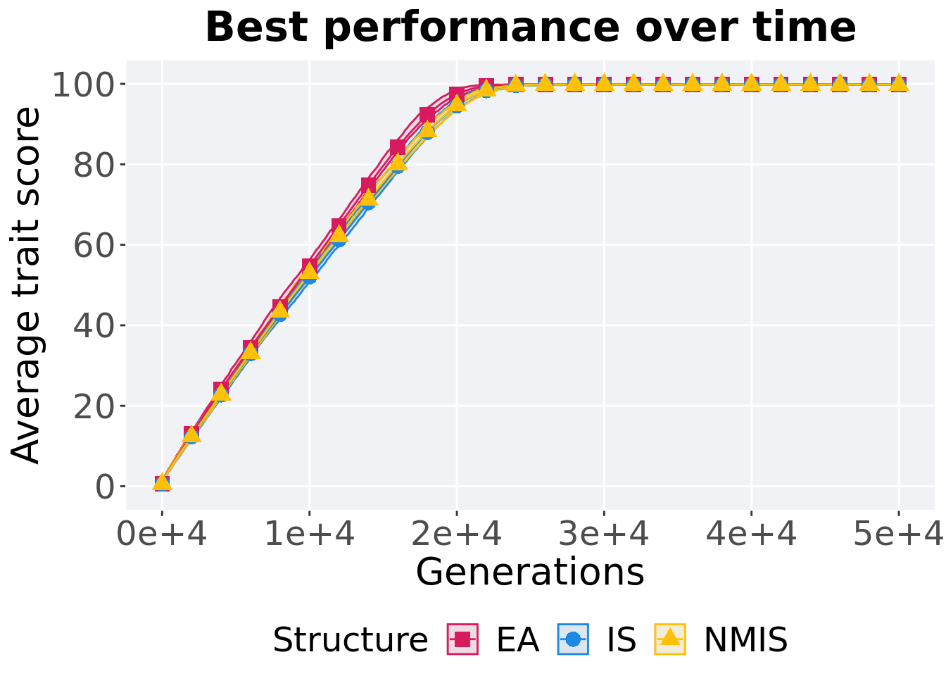

10.4.2 Generation satisfactory solution found

First generation a satisfactory solution is found throughout the 50,000 generations.

filter(mi50_ssf, Diagnostic == 'EXPLOITATION_RATE' & `Selection\nScheme` == 'LEXICASE') %>%
  ggplot(., aes(x = Structure, y = Generations , color = Structure, fill = Structure, shape = Structure)) +
  geom_flat_violin(position = position_nudge(x = .2, y = 0), scale = 'width', alpha = 0.2) +
  geom_point(position = position_jitter(width = .1), size = 1.5, alpha = 1.0) +
  geom_boxplot(color = 'black', width = .2, outlier.shape = NA, alpha = 0.0) +
  scale_y_continuous(
    name="Generation"
  ) +
  scale_x_discrete(
    name="Structure"
  )+
  scale_shape_manual(values=SHAPE)+
  scale_colour_manual(values = cb_palette, ) +
  scale_fill_manual(values = cb_palette) +
  ggtitle('Generation satisfactory solution found')+
  p_theme + coord_flip()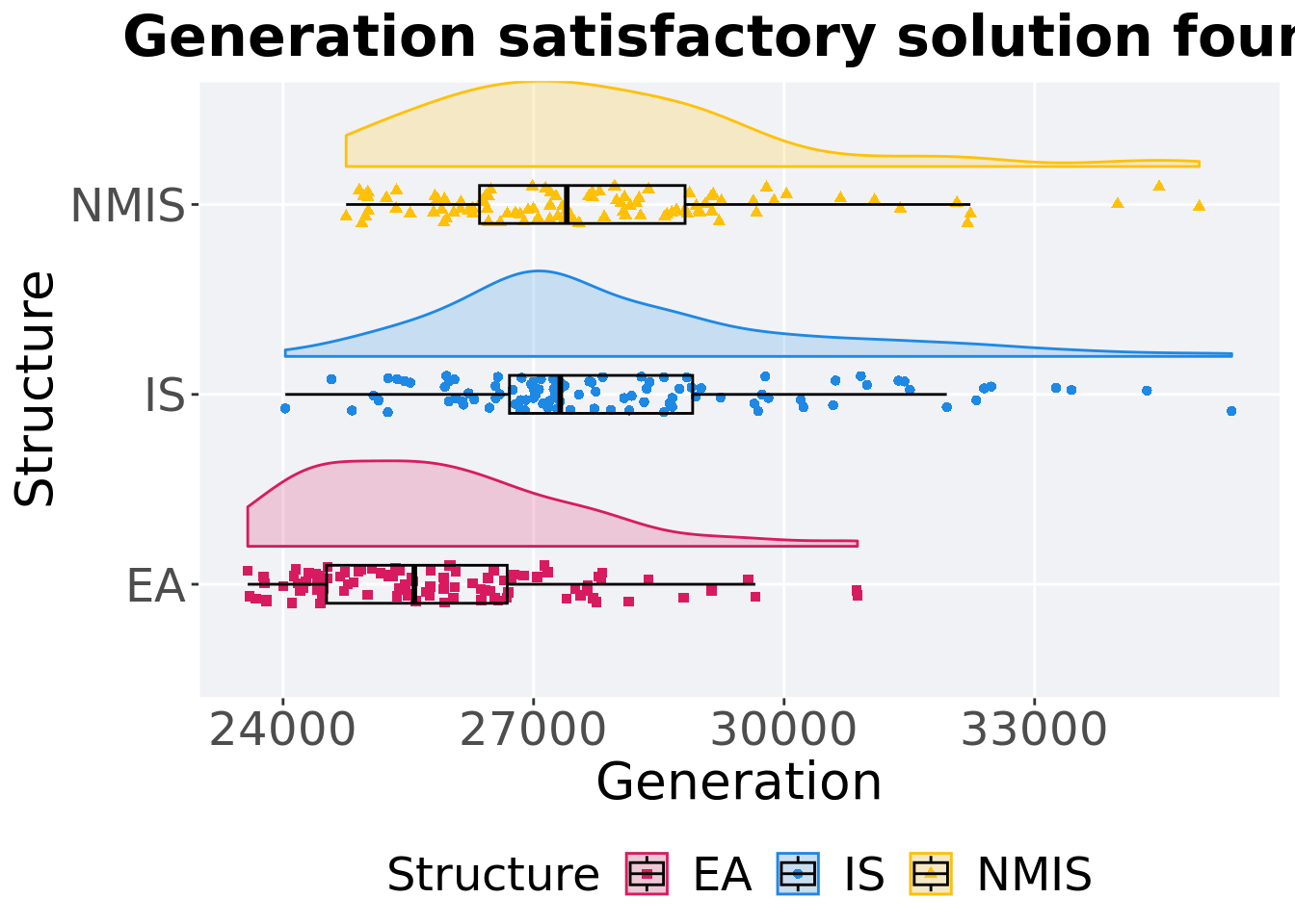

10.4.3 Stats

Summary statistics for the first generation a satisfactory solution is found.

ssf = filter(mi50_ssf, Diagnostic == 'EXPLOITATION_RATE' & `Selection\nScheme` == 'LEXICASE' & Generations < 60000)
ssf %>%
  group_by(Structure) %>%
  dplyr::summarise(
    count = n(),
    na_cnt = sum(is.na(Generations)),
    min = min(Generations, na.rm = TRUE),
    median = median(Generations, na.rm = TRUE),
    mean = mean(Generations, na.rm = TRUE),
    max = max(Generations, na.rm = TRUE),
    IQR = IQR(Generations, na.rm = TRUE)
  )

## # A tibble: 3 x 8
##   Structure count na_cnt   min median   mean   max   IQR
##   <fct>     <int>  <int> <int>  <dbl>  <dbl> <int> <dbl>
## 1 EA          100      0 23577 25572  25861. 30878 2163.
## 2 IS          100      0 24027 27320  28031. 35360 2194.
## 3 NMIS        100      0 24755 27398. 27747. 34971 2462.

Kruskal–Wallis test provides evidence of difference among selection schemes.

kruskal.test(Generations ~ Structure, data = ssf)

## 
##  Kruskal-Wallis rank sum test
## 
## data:  Generations by Structure
## Kruskal-Wallis chi-squared = 69.626, df = 2, p-value = 7.601e-16

Results for post-hoc Wilcoxon rank-sum test with a Bonferroni correction.

pairwise.wilcox.test(x = ssf$Generations, g = ssf$Structure, p.adjust.method = "bonferroni",
                     paired = FALSE, conf.int = FALSE, alternative = 'g')

## 
##  Pairwise comparisons using Wilcoxon rank sum test with continuity correction 
## 
## data:  ssf$Generations and ssf$Structure 
## 
##      EA      IS
## IS   1.2e-13 - 
## NMIS 7.0e-12 1 
## 
## P value adjustment method: bonferroni