Chapter 11 MI50: Ordered exploitation results

Here we present the results for best performances found by each selection scheme replicate on the ordered exploitation diagnostic with configurations presented below. Best performance found refers to the largest average trait score found in a given population. Note that performance values fall between 0.0 and 100.0. For our the configuration of these experiments, we execute migrations every 50 generations and there are 4 islands in a ring topology. When migrations occur, we swap two individuals (same position on each island) and guarantee that no solution can return to the same island.

11.1 Analysis dependencies

library(ggplot2)
library(cowplot)
library(dplyr)
library(PupillometryR)

11.2 Truncation selection

Here we analyze how the different population structures affect truncation selection (size 8) on the ordered exploitation diagnostic.

11.2.1 Performance over time

lines = filter(mi50_over_time, Diagnostic == 'ORDERED_EXPLOITATION' & `Selection\nScheme` == 'TRUNCATION') %>%
  group_by(Structure, Generations) %>%
  dplyr::summarise(
    min = min(pop_fit_max) / DIMENSIONALITY,
    mean = mean(pop_fit_max) / DIMENSIONALITY,
    max = max(pop_fit_max) / DIMENSIONALITY
  )
ggplot(lines, aes(x=Generations, y=mean, group = Structure, fill = Structure, color = Structure, shape = Structure)) +
  geom_ribbon(aes(ymin = min, ymax = max), alpha = 0.1) +
  geom_line(size = 0.5) +
  geom_point(data = filter(lines, Generations %% 2000 == 0), size = 2.5, stroke = 2.0, alpha = 1.0) +
  scale_y_continuous(
    name="Average trait score",
    limits=c(-1, 101),
    breaks=seq(0,100, 20),
    labels=c("0", "20", "40", "60", "80", "100")
  ) +
  scale_x_continuous(
    name="Generations",
    limits=c(0, 50000),
    breaks=c(0, 10000, 20000, 30000, 40000, 50000),
    labels=c("0e+4", "1e+4", "2e+4", "3e+4", "4e+4", "5e+4")

  ) +
  scale_shape_manual(values=SHAPE)+
  scale_colour_manual(values = cb_palette) +
  scale_fill_manual(values = cb_palette) +
  ggtitle("Performance over time") +
  p_theme

11.2.2 Generation satisfactory solution found

First generation a satisfactory solution is found throughout the 50,000 generations.

filter(mi50_ssf, Diagnostic == 'ORDERED_EXPLOITATION' & `Selection\nScheme` == 'TRUNCATION') %>%
  ggplot(., aes(x = Structure, y = Generations , color = Structure, fill = Structure, shape = Structure)) +
  geom_flat_violin(position = position_nudge(x = .2, y = 0), scale = 'width', alpha = 0.2) +
  geom_point(position = position_jitter(width = .1), size = 1.5, alpha = 1.0) +
  geom_boxplot(color = 'black', width = .2, outlier.shape = NA, alpha = 0.0) +
  scale_y_continuous(
    name="Generation"
  ) +
  scale_x_discrete(
    name="Structure"
  )+
  scale_shape_manual(values=SHAPE)+
  scale_colour_manual(values = cb_palette, ) +
  scale_fill_manual(values = cb_palette) +
  ggtitle('Generation satisfactory solution found')+
  p_theme + coord_flip()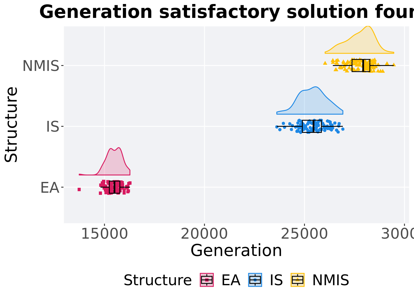

11.2.2.1 Stats

Summary statistics for the first generation a satisfactory solution is found.

ssf = filter(mi50_ssf, Diagnostic == 'ORDERED_EXPLOITATION' & `Selection\nScheme` == 'TRUNCATION' & Generations < 60000)
ssf %>%
  group_by(Structure) %>%
  dplyr::summarise(
    count = n(),
    na_cnt = sum(is.na(Generations)),
    min = min(Generations, na.rm = TRUE),
    median = median(Generations, na.rm = TRUE),
    mean = mean(Generations, na.rm = TRUE),
    max = max(Generations, na.rm = TRUE),
    IQR = IQR(Generations, na.rm = TRUE)
  )

## # A tibble: 3 x 8
##   Structure count na_cnt   min median   mean   max   IQR
##   <fct>     <int>  <int> <int>  <dbl>  <dbl> <int> <dbl>
## 1 EA          100      0 13737 15500. 15493. 16273  526.
## 2 IS          100      0 23617 25453  25405. 26920  950 
## 3 NMIS        100      0 26032 27935  27781. 29465  892.

Kruskal–Wallis test provides evidence of difference among selection schemes.

kruskal.test(Generations ~ Structure, data = ssf)

## 
##  Kruskal-Wallis rank sum test
## 
## data:  Generations by Structure
## Kruskal-Wallis chi-squared = 264.17, df = 2, p-value < 2.2e-16

Results for post-hoc Wilcoxon rank-sum test with a Bonferroni correction.

pairwise.wilcox.test(x = ssf$Generations, g = ssf$Structure, p.adjust.method = "bonferroni",
                     paired = FALSE, conf.int = FALSE, alternative = 'g')

## 
##  Pairwise comparisons using Wilcoxon rank sum test with continuity correction 
## 
## data:  ssf$Generations and ssf$Structure 
## 
##      EA     IS    
## IS   <2e-16 -     
## NMIS <2e-16 <2e-16
## 
## P value adjustment method: bonferroni

11.3 Tournament selection

Here we analyze how the different population structures affect tournament selection (size 8) on the ordered exploitation diagnostic.

11.3.1 Performance over time

lines = filter(mi50_over_time, Diagnostic == 'ORDERED_EXPLOITATION' & `Selection\nScheme` == 'TOURNAMENT') %>%
  group_by(Structure, Generations) %>%
  dplyr::summarise(
    min = min(pop_fit_max) / DIMENSIONALITY,
    mean = mean(pop_fit_max) / DIMENSIONALITY,
    max = max(pop_fit_max) / DIMENSIONALITY
  )
ggplot(lines, aes(x=Generations, y=mean, group = Structure, fill = Structure, color = Structure, shape = Structure)) +
  geom_ribbon(aes(ymin = min, ymax = max), alpha = 0.1) +
  geom_line(size = 0.5) +
  geom_point(data = filter(lines, Generations %% 2000 == 0), size = 2.5, stroke = 2.0, alpha = 1.0) +
  scale_y_continuous(
    name="Average trait score",
    limits=c(-1, 101),
    breaks=seq(0,100, 20),
    labels=c("0", "20", "40", "60", "80", "100")
  ) +
  scale_x_continuous(
    name="Generations",
    limits=c(0, 50000),
    breaks=c(0, 10000, 20000, 30000, 40000, 50000),
    labels=c("0e+4", "1e+4", "2e+4", "3e+4", "4e+4", "5e+4")

  ) +
  scale_shape_manual(values=SHAPE)+
  scale_colour_manual(values = cb_palette) +
  scale_fill_manual(values = cb_palette) +
  ggtitle("Performance over time") +
  p_theme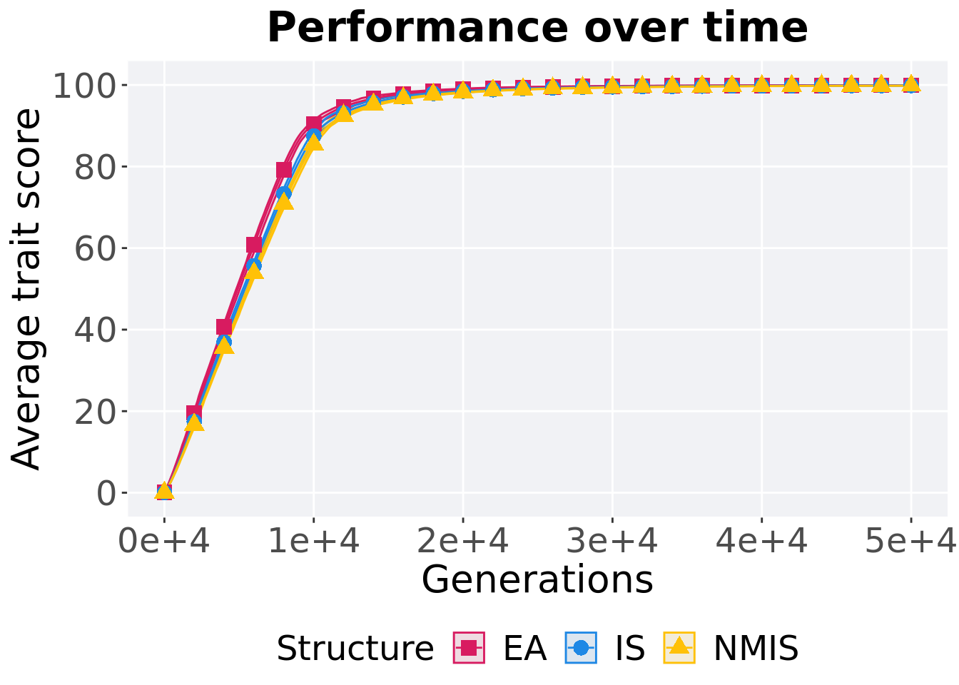

11.3.2 Generation satisfactory solution found

First generation a satisfactory solution is found throughout the 50,000 generations.

filter(mi50_ssf, Diagnostic == 'ORDERED_EXPLOITATION' & `Selection\nScheme` == 'TOURNAMENT') %>%
  ggplot(., aes(x = Structure, y = Generations , color = Structure, fill = Structure, shape = Structure)) +
  geom_flat_violin(position = position_nudge(x = .2, y = 0), scale = 'width', alpha = 0.2) +
  geom_point(position = position_jitter(width = .1), size = 1.5, alpha = 1.0) +
  geom_boxplot(color = 'black', width = .2, outlier.shape = NA, alpha = 0.0) +
  scale_y_continuous(
    name="Generation"
  ) +
  scale_x_discrete(
    name="Structure"
  )+
  scale_shape_manual(values=SHAPE)+
  scale_colour_manual(values = cb_palette, ) +
  scale_fill_manual(values = cb_palette) +
  ggtitle('Generation satisfactory solution found')+
  p_theme + coord_flip()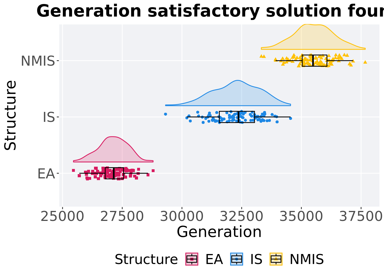

11.3.2.1 Stats

Summary statistics for the first generation a satisfactory solution is found.

ssf = filter(mi50_ssf, Diagnostic == 'ORDERED_EXPLOITATION' & `Selection\nScheme` == 'TOURNAMENT' & Generations < 60000)
ssf %>%
  group_by(Structure) %>%
  dplyr::summarise(
    count = n(),
    na_cnt = sum(is.na(Generations)),
    min = min(Generations, na.rm = TRUE),
    median = median(Generations, na.rm = TRUE),
    mean = mean(Generations, na.rm = TRUE),
    max = max(Generations, na.rm = TRUE),
    IQR = IQR(Generations, na.rm = TRUE)
  )

## # A tibble: 3 x 8
##   Structure count na_cnt   min median   mean   max   IQR
##   <fct>     <int>  <int> <int>  <dbl>  <dbl> <int> <dbl>
## 1 EA          100      0 25458 27144. 27124. 28791  769.
## 2 IS          100      0 29313 32368. 32281. 34547 1474 
## 3 NMIS        100      0 33324 35488. 35510. 37674 1035.

Kruskal–Wallis test provides evidence of difference among selection schemes.

kruskal.test(Generations ~ Structure, data = ssf)

## 
##  Kruskal-Wallis rank sum test
## 
## data:  Generations by Structure
## Kruskal-Wallis chi-squared = 264.58, df = 2, p-value < 2.2e-16

Results for post-hoc Wilcoxon rank-sum test with a Bonferroni correction.

pairwise.wilcox.test(x = ssf$Generations, g = ssf$Structure, p.adjust.method = "bonferroni",
                     paired = FALSE, conf.int = FALSE, alternative = 'g')

## 
##  Pairwise comparisons using Wilcoxon rank sum test with continuity correction 
## 
## data:  ssf$Generations and ssf$Structure 
## 
##      EA     IS    
## IS   <2e-16 -     
## NMIS <2e-16 <2e-16
## 
## P value adjustment method: bonferroni

11.4 Lexicase selection

Here we analyze how the different population structures affect standard lexicase selection on the ordered exploitation diagnostic.

11.4.1 Performance over time

lines = filter(mi50_over_time, Diagnostic == 'ORDERED_EXPLOITATION' & `Selection\nScheme` == 'LEXICASE') %>%
  group_by(Structure, Generations) %>%
  dplyr::summarise(
    min = min(pop_fit_max) / DIMENSIONALITY,
    mean = mean(pop_fit_max) / DIMENSIONALITY,
    max = max(pop_fit_max) / DIMENSIONALITY
  )
ggplot(lines, aes(x=Generations, y=mean, group = Structure, fill = Structure, color = Structure, shape = Structure)) +
  geom_ribbon(aes(ymin = min, ymax = max), alpha = 0.1) +
  geom_line(size = 0.5) +
  geom_point(data = filter(lines, Generations %% 2000 == 0), size = 2.5, stroke = 2.0, alpha = 1.0) +
  scale_y_continuous(
    name="Average trait score",
    limits=c(-1, 101),
    breaks=seq(0,100, 20),
    labels=c("0", "20", "40", "60", "80", "100")
  ) +
  scale_x_continuous(
    name="Generations",
    limits=c(0, 50000),
    breaks=c(0, 10000, 20000, 30000, 40000, 50000),
    labels=c("0e+4", "1e+4", "2e+4", "3e+4", "4e+4", "5e+4")

  ) +
  scale_shape_manual(values=SHAPE)+
  scale_colour_manual(values = cb_palette) +
  scale_fill_manual(values = cb_palette) +
  ggtitle("Performance over time") +
  p_theme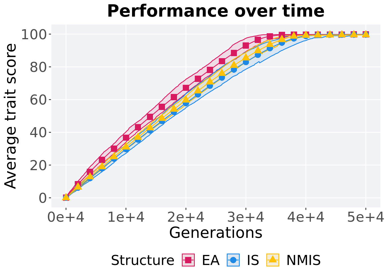

11.4.2 Best performance

First generation a satisfactory solution is found throughout the 50,000 generations.

filter(mi50_best, Diagnostic == 'ORDERED_EXPLOITATION' & `Selection\nScheme` == 'LEXICASE' & VAR == 'pop_fit_max') %>%
  ggplot(., aes(x = Structure, y = VAL / DIMENSIONALITY, color = Structure, fill = Structure, shape = Structure)) +
  geom_flat_violin(position = position_nudge(x = .2, y = 0), scale = 'width', alpha = 0.2) +
  geom_point(position = position_jitter(width = .1), size = 1.5, alpha = 1.0) +
  geom_boxplot(color = 'black', width = .2, outlier.shape = NA, alpha = 0.0) +
  scale_y_continuous(
    name="Average trait score"
  ) +
  scale_x_discrete(
    name="Structure"
  )+
  scale_shape_manual(values=SHAPE)+
  scale_colour_manual(values = cb_palette, ) +
  scale_fill_manual(values = cb_palette) +
  ggtitle('Best performance')+
  p_theme + coord_flip()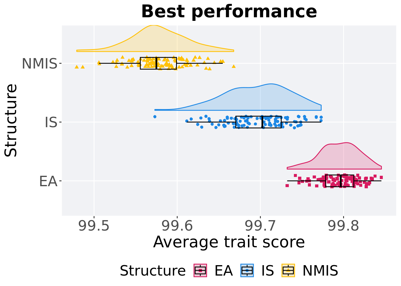

11.4.2.1 Stats

Summary statistics for the first generation a satisfactory solution is found.

performance = filter(mi50_best, Diagnostic == 'ORDERED_EXPLOITATION' & `Selection\nScheme` == 'LEXICASE' & VAR == 'pop_fit_max')
performance %>%
  group_by(Structure) %>%
  dplyr::summarise(
    count = n(),
    na_cnt = sum(is.na(VAL)),
    min = min(VAL, na.rm = TRUE) / DIMENSIONALITY,
    median = median(VAL, na.rm = TRUE) / DIMENSIONALITY,
    mean = mean(VAL, na.rm = TRUE) / DIMENSIONALITY,
    max = max(VAL, na.rm = TRUE) / DIMENSIONALITY,
    IQR = IQR(VAL, na.rm = TRUE) / DIMENSIONALITY
  )

## # A tibble: 3 x 8
##   Structure count na_cnt   min median  mean   max    IQR
##   <fct>     <int>  <int> <dbl>  <dbl> <dbl> <dbl>  <dbl>
## 1 EA          100      0  99.7   99.8  99.8  99.8 0.0338
## 2 IS          100      0  99.6   99.7  99.7  99.8 0.0545
## 3 NMIS        100      0  99.5   99.6  99.6  99.7 0.0435

Kruskal–Wallis test provides evidence of difference among selection schemes.

kruskal.test(VAL ~ Structure, data = performance)

## 
##  Kruskal-Wallis rank sum test
## 
## data:  VAL by Structure
## Kruskal-Wallis chi-squared = 259.68, df = 2, p-value < 2.2e-16

Results for post-hoc Wilcoxon rank-sum test with a Bonferroni correction.

pairwise.wilcox.test(x = performance$VAL, g = performance$Structure, p.adjust.method = "bonferroni",
                     paired = FALSE, conf.int = FALSE, alternative = 'l')

## 
##  Pairwise comparisons using Wilcoxon rank sum test with continuity correction 
## 
## data:  performance$VAL and performance$Structure 
## 
##      EA     IS    
## IS   <2e-16 -     
## NMIS <2e-16 <2e-16
## 
## P value adjustment method: bonferroni

11.4.3 Final performance

First generation a satisfactory solution is found throughout the 50,000 generations.

filter(mi50_over_time, Diagnostic == 'ORDERED_EXPLOITATION' & `Selection\nScheme` == 'LEXICASE' & Generations == 50000) %>%
  ggplot(., aes(x = Structure, y = pop_fit_max / DIMENSIONALITY, color = Structure, fill = Structure, shape = Structure)) +
  geom_flat_violin(position = position_nudge(x = .2, y = 0), scale = 'width', alpha = 0.2) +
  geom_point(position = position_jitter(width = .1), size = 1.5, alpha = 1.0) +
  geom_boxplot(color = 'black', width = .2, outlier.shape = NA, alpha = 0.0) +
  scale_y_continuous(
    name="Average trait score"
  ) +
  scale_x_discrete(
    name="Structure"
  )+
  scale_shape_manual(values=SHAPE)+
  scale_colour_manual(values = cb_palette, ) +
  scale_fill_manual(values = cb_palette) +
  ggtitle('Final performance')+
  p_theme + coord_flip()

11.4.3.1 Stats

Summary statistics for the first generation a satisfactory solution is found.

performance = filter(mi50_over_time, Diagnostic == 'ORDERED_EXPLOITATION' & `Selection\nScheme` == 'LEXICASE' & Generations == 50000)
performance %>%
  group_by(Structure) %>%
  dplyr::summarise(
    count = n(),
    na_cnt = sum(is.na(pop_fit_max)),
    min = min(pop_fit_max / DIMENSIONALITY, na.rm = TRUE),
    median = median(pop_fit_max / DIMENSIONALITY, na.rm = TRUE),
    mean = mean(pop_fit_max / DIMENSIONALITY, na.rm = TRUE),
    max = max(pop_fit_max / DIMENSIONALITY, na.rm = TRUE),
    IQR = IQR(pop_fit_max / DIMENSIONALITY, na.rm = TRUE)
  )

## # A tibble: 3 x 8
##   Structure count na_cnt   min median  mean   max    IQR
##   <fct>     <int>  <int> <dbl>  <dbl> <dbl> <dbl>  <dbl>
## 1 EA          100      0  99.7   99.8  99.8  99.8 0.0338
## 2 IS          100      0  99.6   99.7  99.7  99.8 0.0545
## 3 NMIS        100      0  99.5   99.6  99.6  99.7 0.0435

Kruskal–Wallis test provides evidence of difference among selection schemes.

kruskal.test(pop_fit_max ~ Structure, data = performance)

## 
##  Kruskal-Wallis rank sum test
## 
## data:  pop_fit_max by Structure
## Kruskal-Wallis chi-squared = 259.68, df = 2, p-value < 2.2e-16

Results for post-hoc Wilcoxon rank-sum test with a Bonferroni correction.

pairwise.wilcox.test(x = performance$pop_fit_max, g = performance$Structure, p.adjust.method = "bonferroni",
                     paired = FALSE, conf.int = FALSE, alternative = 'l')

## 
##  Pairwise comparisons using Wilcoxon rank sum test with continuity correction 
## 
## data:  performance$pop_fit_max and performance$Structure 
## 
##      EA     IS    
## IS   <2e-16 -     
## NMIS <2e-16 <2e-16
## 
## P value adjustment method: bonferroni

11.4.4 Generation satisfactory solution found

First generation a satisfactory solution is found throughout the 50,000 generations.

lex_fail = filter(mi50_ssf, Diagnostic == 'ORDERED_EXPLOITATION' & `Selection\nScheme` == 'LEXICASE' & GENERATIONS < Generations)
lex_fail$Generations = 55000
lex_fail$Structure <- factor(lex_fail$Structure, levels = MODEL)

filter(mi50_ssf, Diagnostic == 'ORDERED_EXPLOITATION' & `Selection\nScheme` == 'LEXICASE'& Generations <= GENERATIONS) %>%
  ggplot(., aes(x = Structure, y = Generations, color = Structure, fill = Structure, shape = Structure)) +
    geom_flat_violin(position = position_nudge(x = .2, y = 0), scale = 'width', alpha = 0.2) +
  geom_point(position = position_jitter(width = .1), size = 1.5, alpha = 1.0) +
  geom_boxplot(color = 'black', width = .2, outlier.shape = NA, alpha = 0.0) +
  geom_point(data = lex_fail, aes(x = Structure, y = Generations, color = Structure, fill = Structure, shape = Structure),position = position_jitter(width = .05), size = 2.5) +
  scale_shape_manual(values=SHAPE)+
  scale_y_continuous(
    name="Generations",
    limits=c(30000, 55000),
    breaks=c(30000, 40000, 50000, 55000),
    labels=c("3e+4", "4e+4", "5e+4", "Fail")
  ) +
  scale_x_discrete(
    name="Structure"
  ) +
  scale_colour_manual(values = cb_palette) +
  scale_fill_manual(values = cb_palette) +
  p_theme + coord_flip()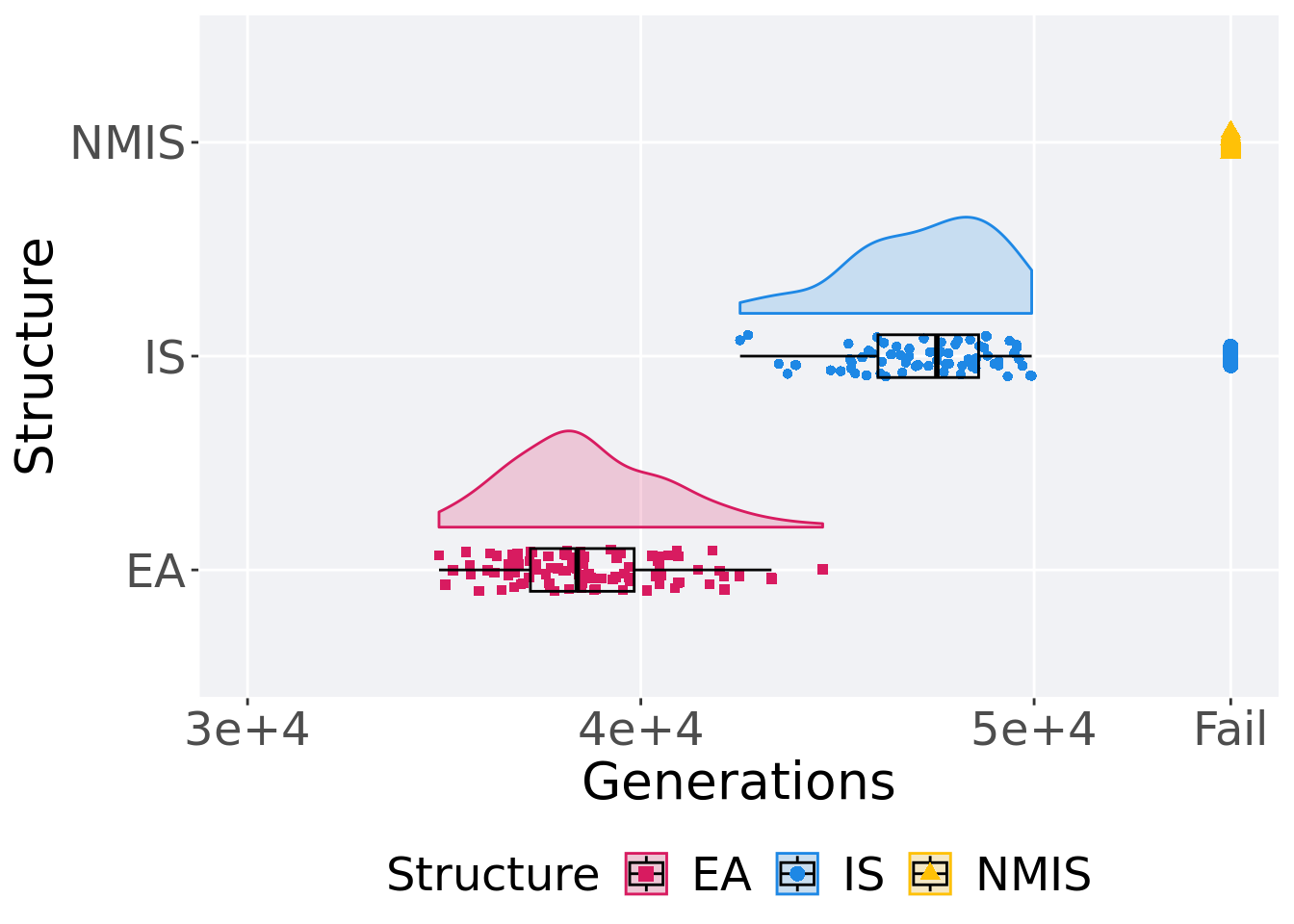

11.4.4.1 Stats

Summary statistics for the first generation a satisfactory solution is found.

ssf = filter(mi50_ssf, Diagnostic == 'ORDERED_EXPLOITATION' & `Selection\nScheme` == 'LEXICASE' & Generations < 60000)
ssf %>%
  group_by(Structure) %>%
  dplyr::summarise(
    count = n(),
    na_cnt = sum(is.na(Generations)),
    min = min(Generations, na.rm = TRUE),
    median = median(Generations, na.rm = TRUE),
    mean = mean(Generations, na.rm = TRUE),
    max = max(Generations, na.rm = TRUE),
    IQR = IQR(Generations, na.rm = TRUE)
  )

## # A tibble: 2 x 8
##   Structure count na_cnt   min median   mean   max   IQR
##   <fct>     <int>  <int> <int>  <dbl>  <dbl> <int> <dbl>
## 1 EA          100      0 34868 38382. 38649. 44624 2638.
## 2 IS           70      0 42523 47526. 47195. 49938 2560.

Kruskal–Wallis test provides evidence of difference among selection schemes.

kruskal.test(Generations ~ Structure, data = ssf)

## 
##  Kruskal-Wallis rank sum test
## 
## data:  Generations by Structure
## Kruskal-Wallis chi-squared = 122.11, df = 1, p-value < 2.2e-16

Results for post-hoc Wilcoxon rank-sum test with a Bonferroni correction.

pairwise.wilcox.test(x = ssf$Generations, g = ssf$Structure, p.adjust.method = "bonferroni",
                     paired = FALSE, conf.int = FALSE, alternative = 'g')

## 
##  Pairwise comparisons using Wilcoxon rank sum test with continuity correction 
## 
## data:  ssf$Generations and ssf$Structure 
## 
##    EA    
## IS <2e-16
## 
## P value adjustment method: bonferroni