Chapter 4 Interval comparison: Contradictory objectives results

Here we present the results for the satisfactory trait corverage and activation gene coverage generated by each selection scheme replicate on the contradictory objectives diagnostic with our base configurations. Note both of these values are gathered at the population-level. Activation gene coverage refers to the count of unique activation genes in a given population; this gives us a range of integers between 0 and 100. Satisfactory trait coverage refers to the count of unique satisfied traits in a given population; this gives us a range of integers between 0 and 100. For our base configuration, there are 4 islands in a ring topology. When migrations occur, two individuals are swapped (same position on each island) and guarantee that no solution can return to its original island.

4.1 Analysis dependencies

library(ggplot2)
library(cowplot)
library(dplyr)
library(PupillometryR)

4.2 Data

base   = filter(base_over_time,   Diagnostic == 'CONTRADICTORY_OBJECTIVES' & Structure == 'IS')
mi50   = filter(mi50_over_time,   Diagnostic == 'CONTRADICTORY_OBJECTIVES' & Structure == 'IS')
mi5000 = filter(mi5000_over_time, Diagnostic == 'CONTRADICTORY_OBJECTIVES' & Structure == 'IS')

base$Interval = '500'
mi50$Interval = '50'
mi5000$Interval = '5000'

df_ot = rbind(base, mi50, mi5000)
df_ot$Interval = factor(df_ot$Interval, levels=c('50','500','5000'))

base = filter(base_best,     Diagnostic == 'CONTRADICTORY_OBJECTIVES' & Structure == 'IS')
mi50 = filter(mi50_best,     Diagnostic == 'CONTRADICTORY_OBJECTIVES' & Structure == 'IS')
mi5000 = filter(mi5000_best, Diagnostic == 'CONTRADICTORY_OBJECTIVES' & Structure == 'IS')

base$Interval = '500'
mi50$Interval = '50'
mi5000$Interval = '5000'

df_best = rbind(mi50,base,mi5000)
df_best$Interval = factor(df_best$Interval, levels = c('50','500','5000'))

4.3 Truncation selection

Here we analyze how the different population structures affect truncation selection (size 8) on the contradictory objectives diagnostic.

4.3.1 Satisfactory trait coverage

Satisfactory trait coverage analysis.

4.3.1.1 Coverage over time

Satisfactory trait coverage over time.

lines = filter(df_ot,`Selection\nScheme` == 'TRUNCATION') %>%
  group_by(Interval, Generations) %>%
  dplyr::summarise(
    min = min(pop_sat_cov),
    mean = mean(pop_sat_cov),
    max = max(pop_sat_cov)
  )

## `summarise()` has grouped output by 'Interval'. You can override using the
## `.groups` argument.

ggplot(lines, aes(x=Generations, y=mean, group = Interval, fill = Interval, color = Interval, shape = Interval)) +
  geom_ribbon(aes(ymin = min, ymax = max), alpha = 0.1) +
  geom_line(size = 0.5) +
  geom_point(data = filter(lines, Generations %% 2000 == 0), size = 1.5, stroke = 2.0, alpha = 1.0) +
  scale_y_continuous(
    name="Coverage"
  ) +
  scale_x_continuous(
    name="Generations",
    limits=c(0, 50000),
    breaks=c(0, 10000, 20000, 30000, 40000, 50000),
    labels=c("0e+4", "1e+4", "2e+4", "3e+4", "4e+4", "5e+4")

  ) +
  scale_shape_manual(values=SHAPE)+
  scale_colour_manual(values = cb_palette_mi) +
  scale_fill_manual(values = cb_palette_mi) +
  ggtitle('Satisfactory trait coverage over time')+
  p_theme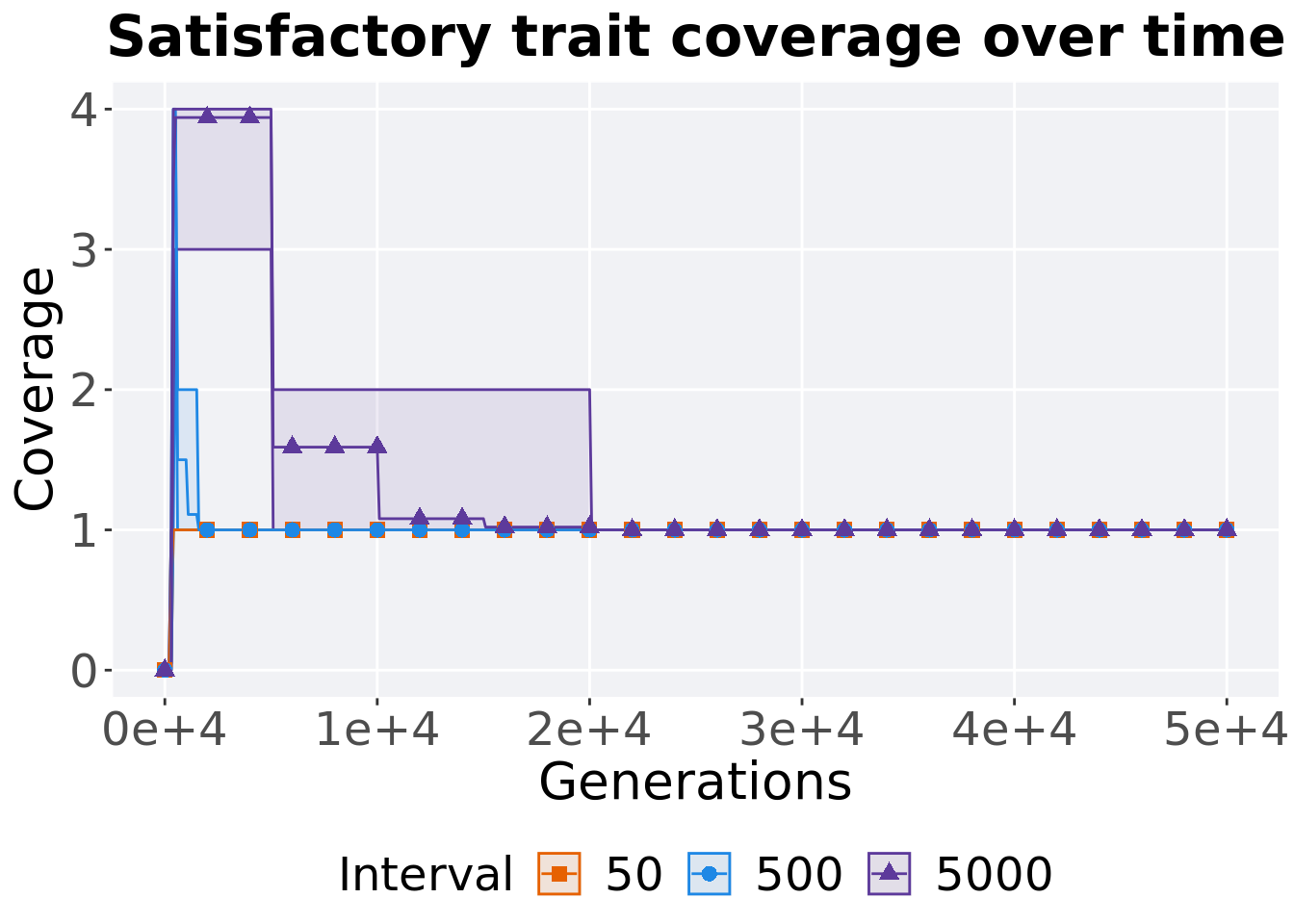

4.3.1.2 Best coverage throughout

Best satisfactory trait coverage throughout 50,000 generations.

### best satisfactory trait coverage throughout
filter(df_best, Diagnostic == 'CONTRADICTORY_OBJECTIVES' & `Selection\nScheme` == 'TRUNCATION' & VAR == 'pop_sat_cov') %>%
  ggplot(., aes(x = Interval, y = VAL, color = Interval, fill = Interval, shape = Interval)) +
  geom_flat_violin(position = position_nudge(x = .2, y = 0), scale = 'width', alpha = 0.2) +
  geom_point(position = position_jitter(height = .05, width = .05), size = 1.5, alpha = 1.0) +
  geom_boxplot(color = 'black', width = .2, outlier.shape = NA, alpha = 0.0) +
  scale_y_continuous(
    name="coverage"
  ) +
  scale_x_discrete(
    name="Interval"
  )+
  scale_shape_manual(values=SHAPE)+
  scale_colour_manual(values = cb_palette_mi, ) +
  scale_fill_manual(values = cb_palette_mi) +
  ggtitle('Best satisfactory trait coverage')+
  p_theme + coord_flip()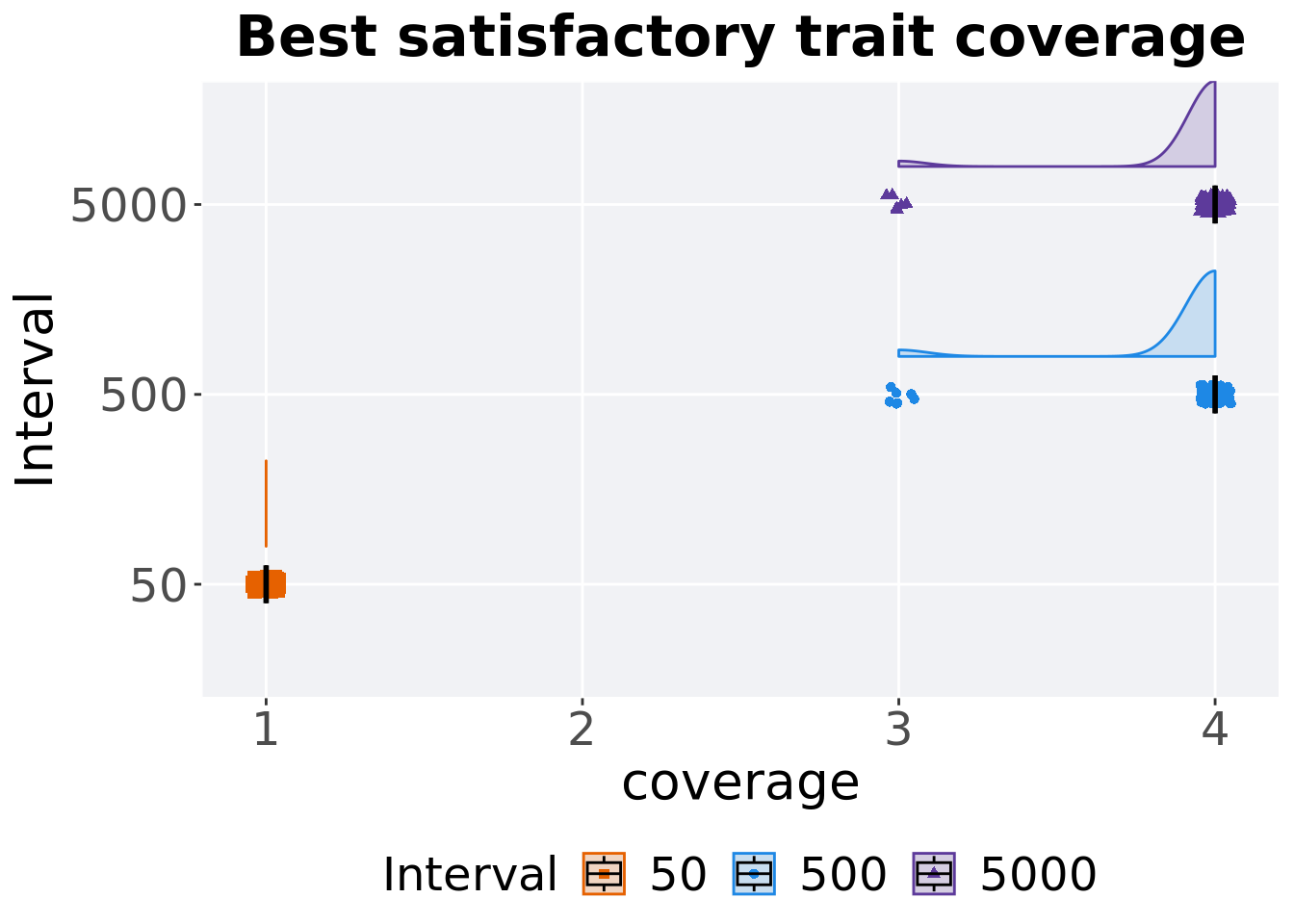

4.3.1.2.1 Stats

Summary statistics for the best satisfactory trait coverage.

### best
coverage = filter(df_best, Diagnostic == 'CONTRADICTORY_OBJECTIVES' & `Selection\nScheme` == 'TRUNCATION' & VAR == 'pop_sat_cov')
coverage %>%
  group_by(Interval) %>%
  dplyr::summarise(
    count = n(),
    na_cnt = sum(is.na(VAL)),
    min = min(VAL, na.rm = TRUE),
    median = median(VAL, na.rm = TRUE),
    mean = mean(VAL, na.rm = TRUE),
    max = max(VAL, na.rm = TRUE),
    IQR = IQR(VAL, na.rm = TRUE)
  )

## # A tibble: 3 x 8
##   Interval count na_cnt   min median  mean   max   IQR
##   <fct>    <int>  <int> <dbl>  <dbl> <dbl> <dbl> <dbl>
## 1 50         100      0     1      1  1        1     0
## 2 500        100      0     3      4  3.93     4     0
## 3 5000       100      0     3      4  3.94     4     0

Kruskal–Wallis test provides evidence of difference among satisfactory trait coverage.

kruskal.test(VAL ~ Interval, data = coverage)

## 
##  Kruskal-Wallis rank sum test
## 
## data:  VAL by Interval
## Kruskal-Wallis chi-squared = 276.6, df = 2, p-value < 2.2e-16

Results for post-hoc Wilcoxon rank-sum test with a Bonferroni correction on satisfactory trait coverage.

pairwise.wilcox.test(x = coverage$VAL, g = coverage$Interval, p.adjust.method = "bonferroni",
                     paired = FALSE, conf.int = FALSE, alternative = 'g')

## 
##  Pairwise comparisons using Wilcoxon rank sum test with continuity correction 
## 
## data:  coverage$VAL and coverage$Interval 
## 
##      50     500
## 500  <2e-16 -  
## 5000 <2e-16 1  
## 
## P value adjustment method: bonferroni

4.3.1.3 End of 50,000 generations

Satisfactory trait coverage in the population at the end of 50,000 generations.

### end of run
filter(df_ot, Diagnostic == 'CONTRADICTORY_OBJECTIVES' & `Selection\nScheme` == 'TRUNCATION' & Generations == 50000) %>%
  ggplot(., aes(x = Interval, y = pop_sat_cov, color = Interval, fill = Interval, shape = Interval)) +
  geom_flat_violin(position = position_nudge(x = .2, y = 0), scale = 'width', alpha = 0.3) +
  geom_point(position = position_jitter(height = .05, width = .05), size = 1.5, alpha = 0.5) +
  geom_boxplot(color = 'black', width = .2, outlier.shape = NA, alpha = 0.0) +
  scale_shape_manual(values=SHAPE)+
  scale_y_continuous(
    name="Coverage"
  ) +
  scale_x_discrete(
    name="Interval"
  ) +
  scale_colour_manual(values = cb_palette_mi) +
  scale_fill_manual(values = cb_palette_mi) +
  ggtitle('Final satisfactory trait coverage')+
  p_theme + coord_flip()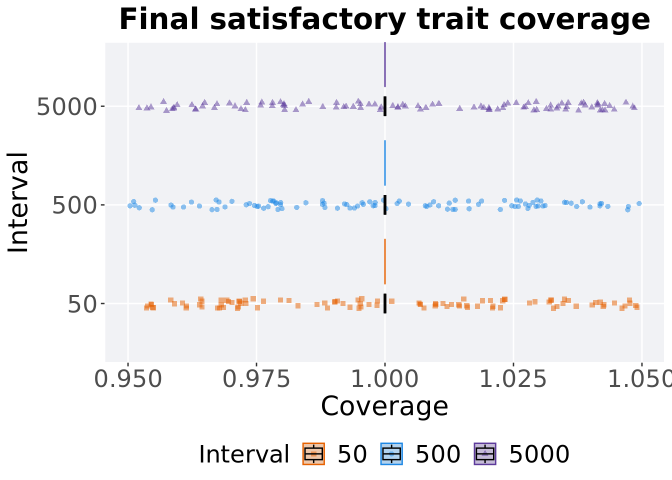

4.3.1.3.1 Stats

Summary statistics for satisfactory trait coverage in the population at the end of 50,000 generations.

### end of run
coverage = filter(df_ot, Diagnostic == 'CONTRADICTORY_OBJECTIVES' & `Selection\nScheme` == 'TRUNCATION' & Generations == 50000)
coverage %>%
  group_by(Interval) %>%
  dplyr::summarise(
    count = n(),
    na_cnt = sum(is.na(pop_sat_cov)),
    min = min(pop_sat_cov, na.rm = TRUE),
    median = median(pop_sat_cov, na.rm = TRUE),
    mean = mean(pop_sat_cov, na.rm = TRUE),
    max = max(pop_sat_cov, na.rm = TRUE),
    IQR = IQR(pop_sat_cov, na.rm = TRUE)
  )

## # A tibble: 3 x 8
##   Interval count na_cnt   min median  mean   max   IQR
##   <fct>    <int>  <int> <int>  <dbl> <dbl> <int> <dbl>
## 1 50         100      0     1      1     1     1     0
## 2 500        100      0     1      1     1     1     0
## 3 5000       100      0     1      1     1     1     0

Kruskal–Wallis test provides evidence of difference among satisfactory trait coverage in the population at the end of 50,000 generations.

kruskal.test(pop_sat_cov ~ Interval, data = coverage)

## 
##  Kruskal-Wallis rank sum test
## 
## data:  pop_sat_cov by Interval
## Kruskal-Wallis chi-squared = NaN, df = 2, p-value = NA

Results for post-hoc Wilcoxon rank-sum test with a Bonferroni correction on satisfactory trait coverage in the population at the end of 50,000 generations.

pairwise.wilcox.test(x = coverage$pop_sat_cov, g = coverage$Interval, p.adjust.method = "bonferroni",
                     paired = FALSE, conf.int = FALSE, alternative = 'g')

## 
##  Pairwise comparisons using Wilcoxon rank sum test with continuity correction 
## 
## data:  coverage$pop_sat_cov and coverage$Interval 
## 
##      50 500
## 500  1  -  
## 5000 1  1  
## 
## P value adjustment method: bonferroni

4.3.2 Activation gene coverage

Activation gene coverage analysis.

4.3.2.1 Coverage over time

Activation gene coverage over time.

# data for lines and shading on plots
lines = filter(df_ot, Diagnostic == 'CONTRADICTORY_OBJECTIVES' & `Selection\nScheme` == 'TRUNCATION') %>%
  group_by(Interval, Generations) %>%
  dplyr::summarise(
    min = min(pop_act_cov),
    mean = mean(pop_act_cov),
    max = max(pop_act_cov)
  )

## `summarise()` has grouped output by 'Interval'. You can override using the
## `.groups` argument.

ggplot(lines, aes(x=Generations, y=mean, group = Interval, fill = Interval, color = Interval, shape = Interval)) +
  geom_ribbon(aes(ymin = min, ymax = max), alpha = 0.1) +
  geom_line(size = 0.5) +
  geom_point(data = filter(lines, Generations %% 2000 == 0), size = 1.5, stroke = 2.0, alpha = 1.0) +
  scale_y_continuous(
    name="Coverage"
  ) +
  scale_x_continuous(
    name="Generations",
    limits=c(0, 50000),
    breaks=c(0, 10000, 20000, 30000, 40000, 50000),
    labels=c("0e+4", "1e+4", "2e+4", "3e+4", "4e+4", "5e+4")

  ) +
  scale_shape_manual(values=SHAPE)+
  scale_colour_manual(values = cb_palette_mi) +
  scale_fill_manual(values = cb_palette_mi) +
  ggtitle('Activation gene coverage over time')+
  p_theme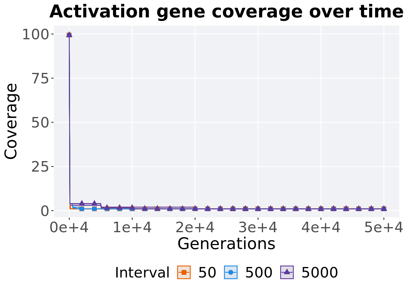

4.3.2.2 End of 50,000 generations

Activation gene coverage in the population at the end of 50,000 generations.

### end of run
filter(df_ot, Diagnostic == 'CONTRADICTORY_OBJECTIVES' & `Selection\nScheme` == 'TRUNCATION' & Generations == 50000) %>%
  ggplot(., aes(x = Interval, y = pop_act_cov, color = Interval, fill = Interval, shape = Interval)) +
  geom_flat_violin(position = position_nudge(x = .2, y = 0), scale = 'width', alpha = 0.3) +
  geom_point(position = position_jitter(height = .05, width = .05), size = 1.5, alpha = 0.5) +
  geom_boxplot(color = 'black', width = .2, outlier.shape = NA, alpha = 0.0) +
  scale_shape_manual(values=SHAPE)+
  scale_y_continuous(
    name="Coverage"
  ) +
  scale_x_discrete(
    name="Interval"
  ) +
  scale_colour_manual(values = cb_palette_mi) +
  scale_fill_manual(values = cb_palette_mi) +
  ggtitle('Final activation gene coverage')+
  p_theme + coord_flip()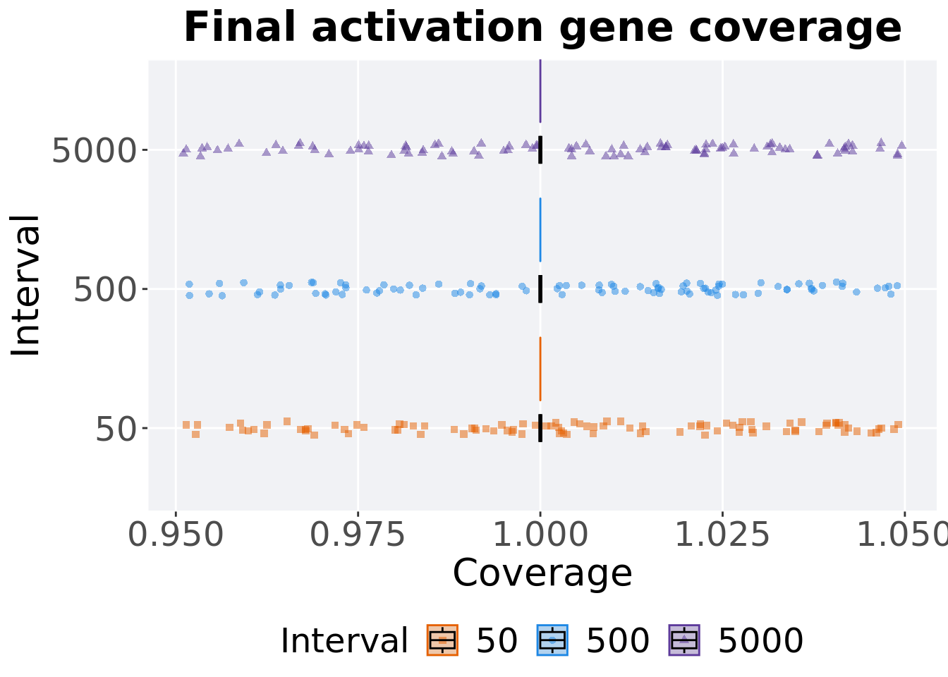

4.3.2.2.1 Stats

Summary statistics for activation gene coverage.

coverage = filter(df_ot, Diagnostic == 'CONTRADICTORY_OBJECTIVES' & `Selection\nScheme` == 'TRUNCATION' & Generations == 50000)
coverage %>%
  group_by(Interval) %>%
  dplyr::summarise(
    count = n(),
    na_cnt = sum(is.na(pop_act_cov)),
    min = min(pop_act_cov, na.rm = TRUE),
    median = median(pop_act_cov, na.rm = TRUE),
    mean = mean(pop_act_cov, na.rm = TRUE),
    max = max(pop_act_cov, na.rm = TRUE),
    IQR = IQR(pop_act_cov, na.rm = TRUE)
  )

## # A tibble: 3 x 8
##   Interval count na_cnt   min median  mean   max   IQR
##   <fct>    <int>  <int> <int>  <dbl> <dbl> <int> <dbl>
## 1 50         100      0     1      1     1     1     0
## 2 500        100      0     1      1     1     1     0
## 3 5000       100      0     1      1     1     1     0

Kruskal–Wallis test provides evidence of difference among activation gene coverage.

kruskal.test(pop_act_cov ~ Interval, data = coverage)

## 
##  Kruskal-Wallis rank sum test
## 
## data:  pop_act_cov by Interval
## Kruskal-Wallis chi-squared = NaN, df = 2, p-value = NA

Results for post-hoc Wilcoxon rank-sum test with a Bonferroni correction on activation gene coverage.

pairwise.wilcox.test(x = coverage$pop_act_cov, g = coverage$Interval, p.adjust.method = "bonferroni",
                     paired = FALSE, conf.int = FALSE, alternative = 'g')

## 
##  Pairwise comparisons using Wilcoxon rank sum test with continuity correction 
## 
## data:  coverage$pop_act_cov and coverage$Interval 
## 
##      50 500
## 500  1  -  
## 5000 1  1  
## 
## P value adjustment method: bonferroni

4.4 Tournament selection

Here we analyze how the different population structures affect tournament selection (size 8) on the contradictory objectives diagnostic.

4.4.1 Satisfactory trait coverage

Satisfactory trait coverage analysis.

4.4.1.1 Coverage over time

Satisfactory trait coverage over time.

lines = filter(df_ot, Diagnostic == 'CONTRADICTORY_OBJECTIVES' & `Selection\nScheme` == 'TOURNAMENT') %>%
  group_by(Interval, Generations) %>%
  dplyr::summarise(
    min = min(pop_sat_cov),
    mean = mean(pop_sat_cov),
    max = max(pop_sat_cov)
  )

## `summarise()` has grouped output by 'Interval'. You can override using the
## `.groups` argument.

ggplot(lines, aes(x=Generations, y=mean, group = Interval, fill = Interval, color = Interval, shape = Interval)) +
  geom_ribbon(aes(ymin = min, ymax = max), alpha = 0.1) +
  geom_line(size = 0.5) +
  geom_point(data = filter(lines, Generations %% 2000 == 0), size = 1.5, stroke = 2.0, alpha = 1.0) +
  scale_y_continuous(
    name="Coverage"
  ) +
  scale_x_continuous(
    name="Generations",
    limits=c(0, 50000),
    breaks=c(0, 10000, 20000, 30000, 40000, 50000),
    labels=c("0e+4", "1e+4", "2e+4", "3e+4", "4e+4", "5e+4")

  ) +
  scale_shape_manual(values=SHAPE)+
  scale_colour_manual(values = cb_palette_mi) +
  scale_fill_manual(values = cb_palette_mi) +
  ggtitle('Satisfactory trait coverage over time')+
  p_theme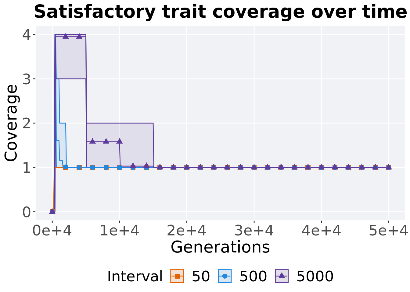

4.4.1.2 Best coverage throughout

Best satisfactory trait coverage throughout 50,000 generations.

### best satisfactory trait coverage throughout
filter(df_best, Diagnostic == 'CONTRADICTORY_OBJECTIVES' & `Selection\nScheme` == 'TOURNAMENT' & VAR == 'pop_sat_cov') %>%
  ggplot(., aes(x = Interval, y = VAL, color = Interval, fill = Interval, shape = Interval)) +
  geom_flat_violin(position = position_nudge(x = .2, y = 0), scale = 'width', alpha = 0.2) +
  geom_point(position = position_jitter(height = .05, width = .05), size = 1.5, alpha = 1.0) +
  geom_boxplot(color = 'black', width = .2, outlier.shape = NA, alpha = 0.0) +
  scale_y_continuous(
    name="coverage"
  ) +
  scale_x_discrete(
    name="Interval"
  )+
  scale_shape_manual(values=SHAPE)+
  scale_colour_manual(values = cb_palette_mi, ) +
  scale_fill_manual(values = cb_palette_mi) +
  ggtitle('Best satisfactory trait coverage')+
  p_theme + coord_flip()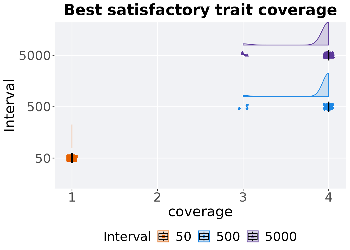

4.4.1.2.1 Stats

Summary statistics for the best satisfactory trait coverage.

### best
coverage = filter(df_best, Diagnostic == 'CONTRADICTORY_OBJECTIVES' & `Selection\nScheme` == 'TOURNAMENT' & VAR == 'pop_sat_cov')
coverage %>%
  group_by(Interval) %>%
  dplyr::summarise(
    count = n(),
    na_cnt = sum(is.na(VAL)),
    min = min(VAL, na.rm = TRUE),
    median = median(VAL, na.rm = TRUE),
    mean = mean(VAL, na.rm = TRUE),
    max = max(VAL, na.rm = TRUE),
    IQR = IQR(VAL, na.rm = TRUE)
  )

## # A tibble: 3 x 8
##   Interval count na_cnt   min median  mean   max   IQR
##   <fct>    <int>  <int> <dbl>  <dbl> <dbl> <dbl> <dbl>
## 1 50         100      0     1      1  1        1     0
## 2 500        100      0     3      4  3.96     4     0
## 3 5000       100      0     3      4  3.95     4     0

Kruskal–Wallis test provides evidence of difference among satisfactory trait coverage.

kruskal.test(VAL ~ Interval, data = coverage)

## 
##  Kruskal-Wallis rank sum test
## 
## data:  VAL by Interval
## Kruskal-Wallis chi-squared = 282.81, df = 2, p-value < 2.2e-16

Results for post-hoc Wilcoxon rank-sum test with a Bonferroni correction on satisfactory trait coverage.

pairwise.wilcox.test(x = coverage$VAL, g = coverage$Interval, p.adjust.method = "bonferroni",
                     paired = FALSE, conf.int = FALSE, alternative = 'g')

## 
##  Pairwise comparisons using Wilcoxon rank sum test with continuity correction 
## 
## data:  coverage$VAL and coverage$Interval 
## 
##      50     500
## 500  <2e-16 -  
## 5000 <2e-16 1  
## 
## P value adjustment method: bonferroni

4.4.1.3 End of 50,000 generations

Satisfactory trait coverage in the population at the end of 50,000 generations.

### end of run
filter(df_ot, Diagnostic == 'CONTRADICTORY_OBJECTIVES' & `Selection\nScheme` == 'TOURNAMENT' & Generations == 50000) %>%
  ggplot(., aes(x = Interval, y = pop_sat_cov, color = Interval, fill = Interval, shape = Interval)) +
  geom_flat_violin(position = position_nudge(x = .2, y = 0), scale = 'width', alpha = 0.3) +
  geom_point(position = position_jitter(height = .05, width = .05), size = 1.5, alpha = 0.5) +
  geom_boxplot(color = 'black', width = .2, outlier.shape = NA, alpha = 0.0) +
  scale_shape_manual(values=SHAPE)+
  scale_y_continuous(
    name="Coverage"
  ) +
  scale_x_discrete(
    name="Interval"
  ) +
  scale_colour_manual(values = cb_palette_mi) +
  scale_fill_manual(values = cb_palette_mi) +
  ggtitle('Final satisfactory trait coverage')+
  p_theme + coord_flip()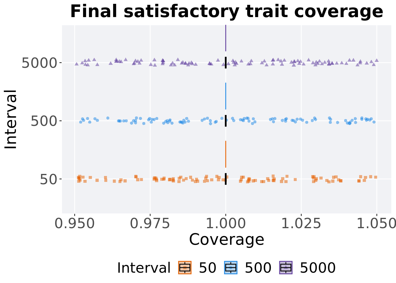

4.4.1.3.1 Stats

Summary statistics for satisfactory trait coverage in the population at the end of 50,000 generations.

### end of run
coverage = filter(df_ot, Diagnostic == 'CONTRADICTORY_OBJECTIVES' & `Selection\nScheme` == 'TOURNAMENT' & Generations == 50000)
coverage %>%
  group_by(Interval) %>%
  dplyr::summarise(
    count = n(),
    na_cnt = sum(is.na(pop_sat_cov)),
    min = min(pop_sat_cov, na.rm = TRUE),
    median = median(pop_sat_cov, na.rm = TRUE),
    mean = mean(pop_sat_cov, na.rm = TRUE),
    max = max(pop_sat_cov, na.rm = TRUE),
    IQR = IQR(pop_sat_cov, na.rm = TRUE)
  )

## # A tibble: 3 x 8
##   Interval count na_cnt   min median  mean   max   IQR
##   <fct>    <int>  <int> <int>  <dbl> <dbl> <int> <dbl>
## 1 50         100      0     1      1     1     1     0
## 2 500        100      0     1      1     1     1     0
## 3 5000       100      0     1      1     1     1     0

Kruskal–Wallis test provides evidence of difference among satisfactory trait coverage in the population at the end of 50,000 generations.

kruskal.test(pop_sat_cov ~ Interval, data = coverage)

## 
##  Kruskal-Wallis rank sum test
## 
## data:  pop_sat_cov by Interval
## Kruskal-Wallis chi-squared = NaN, df = 2, p-value = NA

Results for post-hoc Wilcoxon rank-sum test with a Bonferroni correction on satisfactory trait coverage in the population at the end of 50,000 generations.

pairwise.wilcox.test(x = coverage$pop_sat_cov, g = coverage$Interval, p.adjust.method = "bonferroni",
                     paired = FALSE, conf.int = FALSE, alternative = 'g')

## 
##  Pairwise comparisons using Wilcoxon rank sum test with continuity correction 
## 
## data:  coverage$pop_sat_cov and coverage$Interval 
## 
##      50 500
## 500  1  -  
## 5000 1  1  
## 
## P value adjustment method: bonferroni

4.4.2 Activation gene coverage

Activation gene coverage analysis.

4.4.2.1 Coverage over time

Activation gene coverage over time.

# data for lines and shading on plots
lines = filter(df_ot, Diagnostic == 'CONTRADICTORY_OBJECTIVES' & `Selection\nScheme` == 'TOURNAMENT') %>%
  group_by(Interval, Generations) %>%
  dplyr::summarise(
    min = min(pop_act_cov),
    mean = mean(pop_act_cov),
    max = max(pop_act_cov)
  )

## `summarise()` has grouped output by 'Interval'. You can override using the
## `.groups` argument.

ggplot(lines, aes(x=Generations, y=mean, group = Interval, fill = Interval, color = Interval, shape = Interval)) +
  geom_ribbon(aes(ymin = min, ymax = max), alpha = 0.1) +
  geom_line(size = 0.5) +
  geom_point(data = filter(lines, Generations %% 2000 == 0), size = 1.5, stroke = 2.0, alpha = 1.0) +
  scale_y_continuous(
    name="Coverage"
  ) +
  scale_x_continuous(
    name="Generations",
    limits=c(0, 50000),
    breaks=c(0, 10000, 20000, 30000, 40000, 50000),
    labels=c("0e+4", "1e+4", "2e+4", "3e+4", "4e+4", "5e+4")

  ) +
  scale_shape_manual(values=SHAPE)+
  scale_colour_manual(values = cb_palette_mi) +
  scale_fill_manual(values = cb_palette_mi) +
  ggtitle('Activation gene coverage over time')+
  p_theme

4.4.2.2 End of 50,000 generations

Activation gene coverage in the population at the end of 50,000 generations.

### end of run
filter(df_ot, Diagnostic == 'CONTRADICTORY_OBJECTIVES' & `Selection\nScheme` == 'TOURNAMENT' & Generations == 50000) %>%
  ggplot(., aes(x = Interval, y = pop_act_cov, color = Interval, fill = Interval, shape = Interval)) +
  geom_flat_violin(position = position_nudge(x = .2, y = 0), scale = 'width', alpha = 0.3) +
  geom_point(position = position_jitter(height = .05, width = .05), size = 1.5, alpha = 0.5) +
  geom_boxplot(color = 'black', width = .2, outlier.shape = NA, alpha = 0.0) +
  scale_shape_manual(values=SHAPE)+
  scale_y_continuous(
    name="Coverage"
  ) +
  scale_x_discrete(
    name="Interval"
  ) +
  scale_colour_manual(values = cb_palette_mi) +
  scale_fill_manual(values = cb_palette_mi) +
  ggtitle('Final activation gene coverage')+
  p_theme + coord_flip()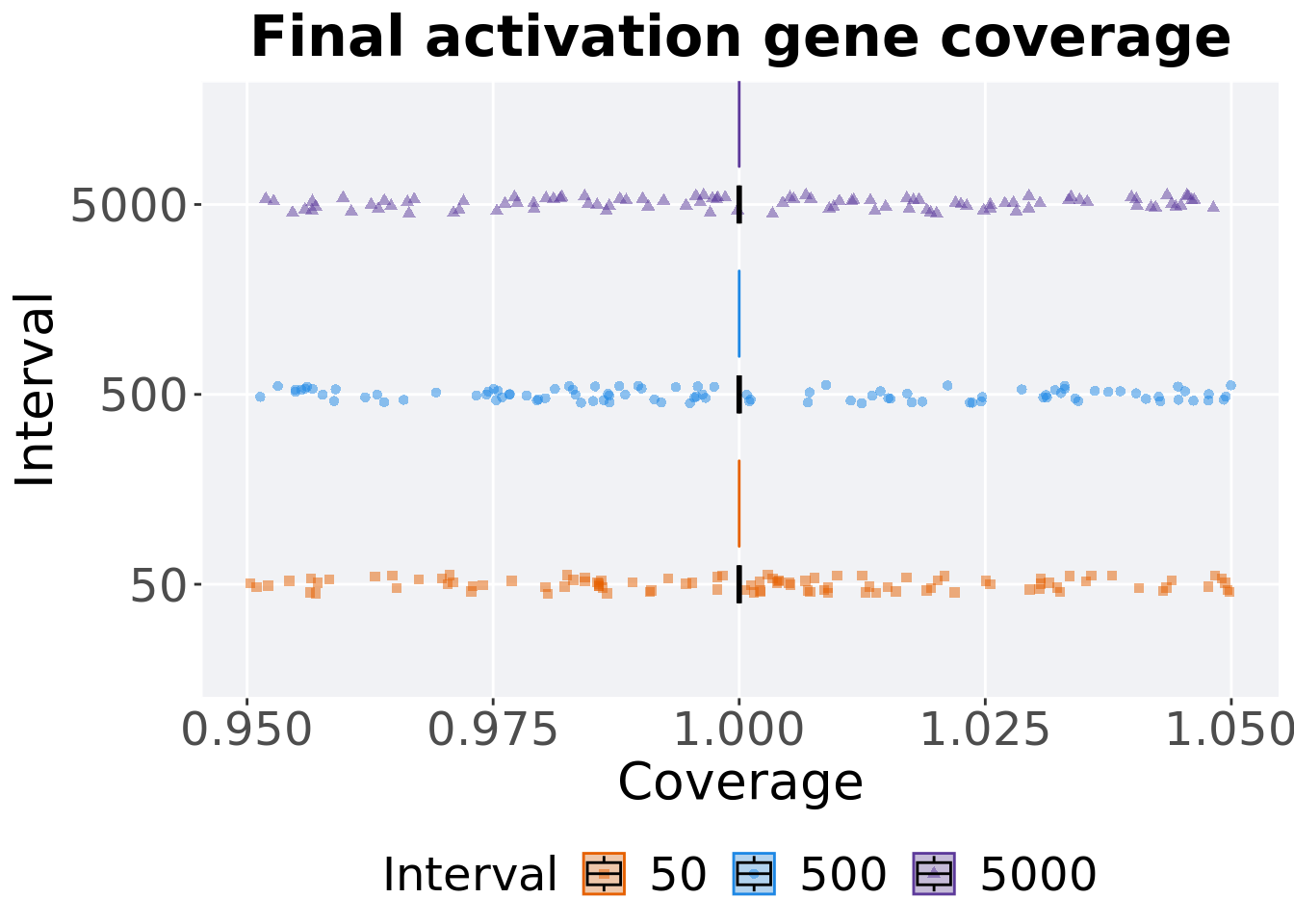

4.4.2.2.1 Stats

Summary statistics for activation gene coverage.

coverage = filter(df_ot, Diagnostic == 'CONTRADICTORY_OBJECTIVES' & `Selection\nScheme` == 'TOURNAMENT' & Generations == 50000)
coverage %>%
  group_by(Interval) %>%
  dplyr::summarise(
    count = n(),
    na_cnt = sum(is.na(pop_act_cov)),
    min = min(pop_act_cov, na.rm = TRUE),
    median = median(pop_act_cov, na.rm = TRUE),
    mean = mean(pop_act_cov, na.rm = TRUE),
    max = max(pop_act_cov, na.rm = TRUE),
    IQR = IQR(pop_act_cov, na.rm = TRUE)
  )

## # A tibble: 3 x 8
##   Interval count na_cnt   min median  mean   max   IQR
##   <fct>    <int>  <int> <int>  <dbl> <dbl> <int> <dbl>
## 1 50         100      0     1      1     1     1     0
## 2 500        100      0     1      1     1     1     0
## 3 5000       100      0     1      1     1     1     0

Kruskal–Wallis test provides evidence of difference among activation gene coverage.

kruskal.test(pop_act_cov ~ Interval, data = coverage)

## 
##  Kruskal-Wallis rank sum test
## 
## data:  pop_act_cov by Interval
## Kruskal-Wallis chi-squared = NaN, df = 2, p-value = NA

Results for post-hoc Wilcoxon rank-sum test with a Bonferroni correction on activation gene coverage.

pairwise.wilcox.test(x = coverage$pop_act_cov, g = coverage$Interval, p.adjust.method = "bonferroni",
                     paired = FALSE, conf.int = FALSE, alternative = 'g')

## 
##  Pairwise comparisons using Wilcoxon rank sum test with continuity correction 
## 
## data:  coverage$pop_act_cov and coverage$Interval 
## 
##      50 500
## 500  1  -  
## 5000 1  1  
## 
## P value adjustment method: bonferroni

4.5 Lexicase selection

Here we analyze how the different population structures affect standard lexicase selection on the contradictory objectives diagnostic.

4.5.1 Satisfactory trait coverage

Satisfactory trait coverage analysis.

4.5.1.1 Coverage over time

Satisfactory trait coverage over time.

lines = filter(df_ot, Diagnostic == 'CONTRADICTORY_OBJECTIVES' & `Selection\nScheme` == 'LEXICASE') %>%
  group_by(Interval, Generations) %>%
  dplyr::summarise(
    min = min(pop_sat_cov),
    mean = mean(pop_sat_cov),
    max = max(pop_sat_cov)
  )

## `summarise()` has grouped output by 'Interval'. You can override using the
## `.groups` argument.

ggplot(lines, aes(x=Generations, y=mean, group = Interval, fill = Interval, color = Interval, shape = Interval)) +
  geom_ribbon(aes(ymin = min, ymax = max), alpha = 0.1) +
  geom_line(size = 0.5) +
  geom_point(data = filter(lines, Generations %% 2000 == 0), size = 1.5, stroke = 2.0, alpha = 1.0) +
  scale_y_continuous(
    name="Coverage"
  ) +
  scale_x_continuous(
    name="Generations",
    limits=c(0, 50000),
    breaks=c(0, 10000, 20000, 30000, 40000, 50000),
    labels=c("0e+4", "1e+4", "2e+4", "3e+4", "4e+4", "5e+4")

  ) +
  scale_shape_manual(values=SHAPE)+
  scale_colour_manual(values = cb_palette_mi) +
  scale_fill_manual(values = cb_palette_mi) +
  ggtitle('Satisfactory trait coverage over time')+
  p_theme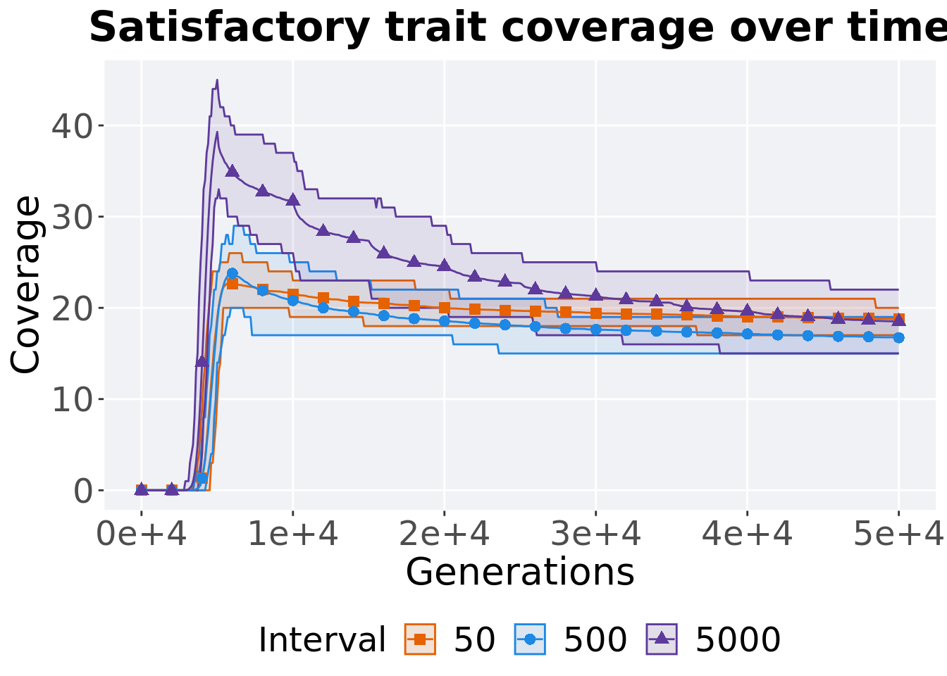

4.5.1.2 Best coverage throughout

Best satisfactory trait coverage throughout 50,000 generations.

### best satisfactory trait coverage throughout
filter(df_best, Diagnostic == 'CONTRADICTORY_OBJECTIVES' & `Selection\nScheme` == 'LEXICASE' & VAR == 'pop_sat_cov') %>%
  ggplot(., aes(x = Interval, y = VAL, color = Interval, fill = Interval, shape = Interval)) +
  geom_flat_violin(position = position_nudge(x = .2, y = 0), scale = 'width', alpha = 0.2) +
  geom_point(position = position_jitter(height = .05, width = .05), size = 1.5, alpha = 1.0) +
  geom_boxplot(color = 'black', width = .2, outlier.shape = NA, alpha = 0.0) +
  scale_y_continuous(
    name="coverage"
  ) +
  scale_x_discrete(
    name="Interval"
  )+
  scale_shape_manual(values=SHAPE)+
  scale_colour_manual(values = cb_palette_mi, ) +
  scale_fill_manual(values = cb_palette_mi) +
  ggtitle('Best satisfactory trait coverage')+
  p_theme + coord_flip()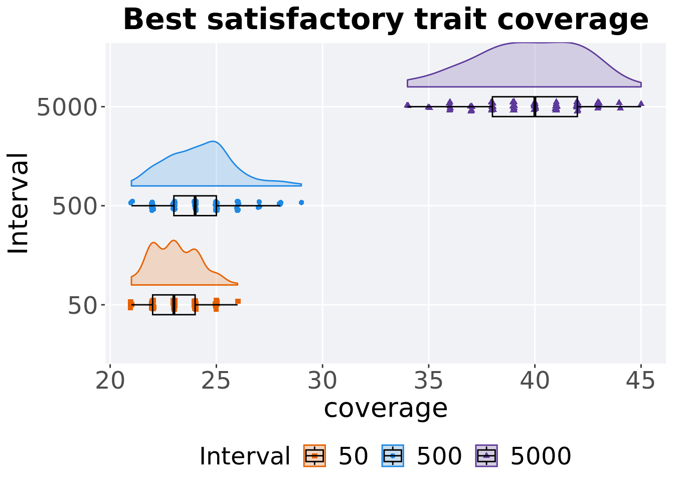

4.5.1.2.1 Stats

Summary statistics for the best satisfactory trait coverage.

### best
coverage = filter(df_best, Diagnostic == 'CONTRADICTORY_OBJECTIVES' & `Selection\nScheme` == 'LEXICASE' & VAR == 'pop_sat_cov')
coverage$Interval = factor(coverage$Interval, levels=c('50','500','5000'))
coverage %>%
  group_by(Interval) %>%
  dplyr::summarise(
    count = n(),
    na_cnt = sum(is.na(VAL)),
    min = min(VAL, na.rm = TRUE),
    median = median(VAL, na.rm = TRUE),
    mean = mean(VAL, na.rm = TRUE),
    max = max(VAL, na.rm = TRUE),
    IQR = IQR(VAL, na.rm = TRUE)
  )

## # A tibble: 3 x 8
##   Interval count na_cnt   min median  mean   max   IQR
##   <fct>    <int>  <int> <dbl>  <dbl> <dbl> <dbl> <dbl>
## 1 50         100      0    21     23  23.0    26     2
## 2 500        100      0    21     24  24.2    29     2
## 3 5000       100      0    34     40  39.7    45     4

Kruskal–Wallis test provides evidence of difference among satisfactory trait coverage.

kruskal.test(VAL ~ Interval, data = coverage)

## 
##  Kruskal-Wallis rank sum test
## 
## data:  VAL by Interval
## Kruskal-Wallis chi-squared = 216.13, df = 2, p-value < 2.2e-16

Results for post-hoc Wilcoxon rank-sum test with a Bonferroni correction on satisfactory trait coverage.

pairwise.wilcox.test(x = coverage$VAL, g = coverage$Interval, p.adjust.method = "bonferroni",
                     paired = FALSE, conf.int = FALSE, alternative = 'g')

## 
##  Pairwise comparisons using Wilcoxon rank sum test with continuity correction 
## 
## data:  coverage$VAL and coverage$Interval 
## 
##      50      500    
## 500  1.8e-08 -      
## 5000 < 2e-16 < 2e-16
## 
## P value adjustment method: bonferroni

4.5.1.3 End of 50,000 generations

Satisfactory trait coverage in the population at the end of 50,000 generations.

### end of run
filter(df_ot, Diagnostic == 'CONTRADICTORY_OBJECTIVES' & `Selection\nScheme` == 'LEXICASE' & Generations == 50000) %>%
  ggplot(., aes(x = Interval, y = pop_sat_cov, color = Interval, fill = Interval, shape = Interval)) +
  geom_flat_violin(position = position_nudge(x = .2, y = 0), scale = 'width', alpha = 0.3) +
  geom_point(position = position_jitter(height = .05, width = .05), size = 1.5, alpha = 0.5) +
  geom_boxplot(color = 'black', width = .2, outlier.shape = NA, alpha = 0.0) +
  scale_shape_manual(values=SHAPE)+
  scale_y_continuous(
    name="Coverage"
  ) +
  scale_x_discrete(
    name="Interval"
  ) +
  scale_colour_manual(values = cb_palette_mi) +
  scale_fill_manual(values = cb_palette_mi) +
  ggtitle('Final satisfactory trait coverage')+
  p_theme + coord_flip()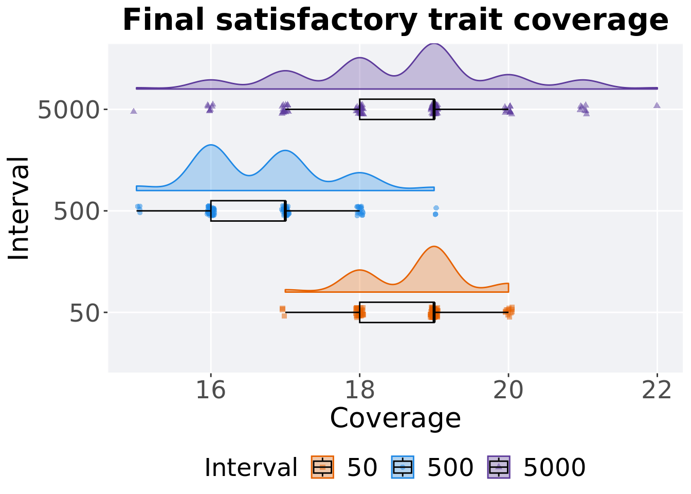

4.5.1.3.1 Stats

Summary statistics for satisfactory trait coverage in the population at the end of 50,000 generations.

### end of run
coverage = filter(df_ot, Diagnostic == 'CONTRADICTORY_OBJECTIVES' & `Selection\nScheme` == 'LEXICASE' & Generations == 50000)
coverage$Interval = factor(coverage$Interval, levels=c('500','50','5000'))
coverage %>%
  group_by(Interval) %>%
  dplyr::summarise(
    count = n(),
    na_cnt = sum(is.na(pop_sat_cov)),
    min = min(pop_sat_cov, na.rm = TRUE),
    median = median(pop_sat_cov, na.rm = TRUE),
    mean = mean(pop_sat_cov, na.rm = TRUE),
    max = max(pop_sat_cov, na.rm = TRUE),
    IQR = IQR(pop_sat_cov, na.rm = TRUE)
  )

## # A tibble: 3 x 8
##   Interval count na_cnt   min median  mean   max   IQR
##   <fct>    <int>  <int> <int>  <dbl> <dbl> <int> <dbl>
## 1 500        100      0    15     17  16.7    19     1
## 2 50         100      0    17     19  18.8    20     1
## 3 5000       100      0    15     19  18.5    22     1

Kruskal–Wallis test provides evidence of difference among satisfactory trait coverage in the population at the end of 50,000 generations.

kruskal.test(pop_sat_cov ~ Interval, data = coverage)

## 
##  Kruskal-Wallis rank sum test
## 
## data:  pop_sat_cov by Interval
## Kruskal-Wallis chi-squared = 139.49, df = 2, p-value < 2.2e-16

Results for post-hoc Wilcoxon rank-sum test with a Bonferroni correction on satisfactory trait coverage in the population at the end of 50,000 generations.

pairwise.wilcox.test(x = coverage$pop_sat_cov, g = coverage$Interval, p.adjust.method = "bonferroni",
                     paired = FALSE, conf.int = FALSE, alternative = 'g')

## 
##  Pairwise comparisons using Wilcoxon rank sum test with continuity correction 
## 
## data:  coverage$pop_sat_cov and coverage$Interval 
## 
##      500    50
## 50   <2e-16 - 
## 5000 <2e-16 1 
## 
## P value adjustment method: bonferroni

4.5.2 Activation gene coverage

Activation gene coverage analysis.

4.5.2.1 Coverage over time

Activation gene coverage over time.

# data for lines and shading on plots
lines = filter(df_ot, Diagnostic == 'CONTRADICTORY_OBJECTIVES' & `Selection\nScheme` == 'LEXICASE') %>%
  group_by(Interval, Generations) %>%
  dplyr::summarise(
    min = min(pop_act_cov),
    mean = mean(pop_act_cov),
    max = max(pop_act_cov)
  )

## `summarise()` has grouped output by 'Interval'. You can override using the
## `.groups` argument.

ggplot(lines, aes(x=Generations, y=mean, group = Interval, fill = Interval, color = Interval, shape = Interval)) +
  geom_ribbon(aes(ymin = min, ymax = max), alpha = 0.1) +
  geom_line(size = 0.5) +
  geom_point(data = filter(lines, Generations %% 2000 == 0), size = 1.5, stroke = 2.0, alpha = 1.0) +
  scale_y_continuous(
    name="Coverage"
  ) +
  scale_x_continuous(
    name="Generations",
    limits=c(0, 50000),
    breaks=c(0, 10000, 20000, 30000, 40000, 50000),
    labels=c("0e+4", "1e+4", "2e+4", "3e+4", "4e+4", "5e+4")

  ) +
  scale_shape_manual(values=SHAPE)+
  scale_colour_manual(values = cb_palette_mi) +
  scale_fill_manual(values = cb_palette_mi) +
  ggtitle('Activation gene coverage over time')+
  p_theme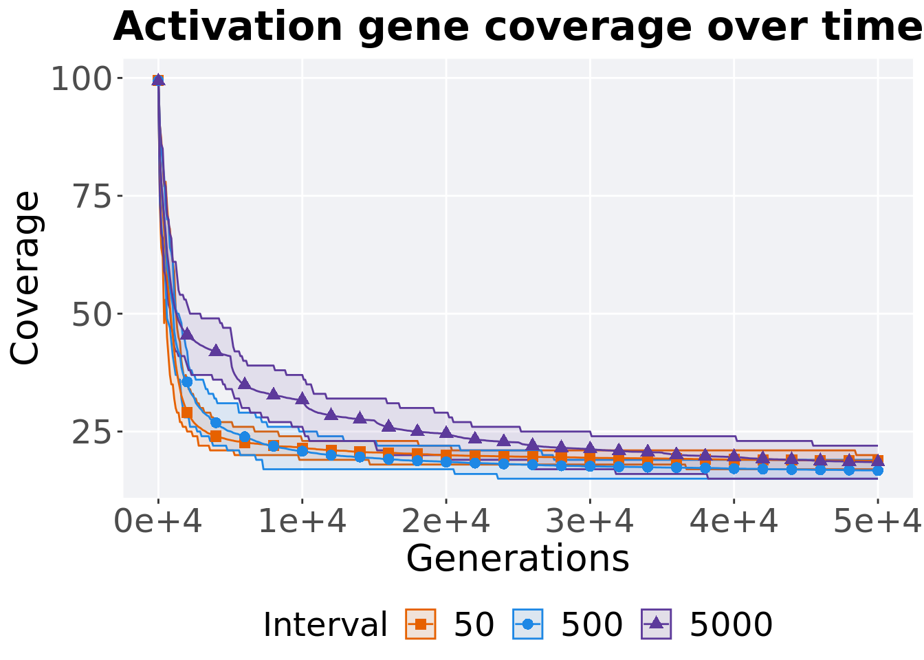

4.5.2.2 End of 50,000 generations

Activation gene coverage in the population at the end of 50,000 generations.

### end of run
filter(df_ot, Diagnostic == 'CONTRADICTORY_OBJECTIVES' & `Selection\nScheme` == 'LEXICASE' & Generations == 50000) %>%
  ggplot(., aes(x = Interval, y = pop_act_cov, color = Interval, fill = Interval, shape = Interval)) +
  geom_flat_violin(position = position_nudge(x = .2, y = 0), scale = 'width', alpha = 0.3) +
  geom_point(position = position_jitter(height = .05, width = .05), size = 1.5, alpha = 0.5) +
  geom_boxplot(color = 'black', width = .2, outlier.shape = NA, alpha = 0.0) +
  scale_shape_manual(values=SHAPE)+
  scale_y_continuous(
    name="Coverage"
  ) +
  scale_x_discrete(
    name="Interval"
  ) +
  scale_colour_manual(values = cb_palette_mi) +
  scale_fill_manual(values = cb_palette_mi) +
  ggtitle('Final activation gene coverage')+
  p_theme + coord_flip()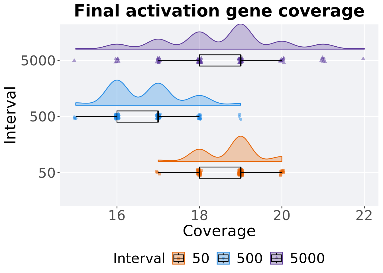

4.5.2.2.1 Stats

Summary statistics for activation gene coverage.

coverage = filter(df_ot, Diagnostic == 'CONTRADICTORY_OBJECTIVES' & `Selection\nScheme` == 'LEXICASE' & Generations == 50000)
coverage$Interval = factor(coverage$Interval, levels=c('500','50','5000'))
coverage %>%
  group_by(Interval) %>%
  dplyr::summarise(
    count = n(),
    na_cnt = sum(is.na(pop_act_cov)),
    min = min(pop_act_cov, na.rm = TRUE),
    median = median(pop_act_cov, na.rm = TRUE),
    mean = mean(pop_act_cov, na.rm = TRUE),
    max = max(pop_act_cov, na.rm = TRUE),
    IQR = IQR(pop_act_cov, na.rm = TRUE)
  )

## # A tibble: 3 x 8
##   Interval count na_cnt   min median  mean   max   IQR
##   <fct>    <int>  <int> <int>  <dbl> <dbl> <int> <dbl>
## 1 500        100      0    15     17  16.7    19     1
## 2 50         100      0    17     19  18.8    20     1
## 3 5000       100      0    15     19  18.5    22     1

Kruskal–Wallis test provides evidence of difference among activation gene coverage.

kruskal.test(pop_act_cov ~ Interval, data = coverage)

## 
##  Kruskal-Wallis rank sum test
## 
## data:  pop_act_cov by Interval
## Kruskal-Wallis chi-squared = 139.49, df = 2, p-value < 2.2e-16

Results for post-hoc Wilcoxon rank-sum test with a Bonferroni correction on activation gene coverage.

pairwise.wilcox.test(x = coverage$pop_act_cov, g = coverage$Interval, p.adjust.method = "bonferroni",
                     paired = FALSE, conf.int = FALSE, alternative = 'g')

## 
##  Pairwise comparisons using Wilcoxon rank sum test with continuity correction 
## 
## data:  coverage$pop_act_cov and coverage$Interval 
## 
##      500    50
## 50   <2e-16 - 
## 5000 <2e-16 1 
## 
## P value adjustment method: bonferroni