Chapter 7 Tournament selection

We present the results from our parameter sweeep on tournament selection. 50 replicates are conducted for each tournament size T parameter value explored.

library(ggplot2)
library(cowplot)
library(dplyr)
library(PupillometryR)

7.1 Exploitation rate results

Here we present the results for best performances found by each tournament selection value replicate on the exploitation rate diagnostic.

7.1.1 Performance over time

Performance over time.

lines = filter(tor_ot, diagnostic == 'exploitation_rate') %>%
        group_by(T, gen) %>%
          dplyr::summarise(
            min = min(pop_fit_max),
            mean = mean(pop_fit_max),
            max = max(pop_fit_max)
          )

## `summarise()` has grouped output by 'T'. You can override using the `.groups`
## argument.

ggplot(lines, aes(x=gen, y=mean / DIMENSIONALITY, group = T, fill = T, color = T, shape = T)) +
  geom_ribbon(aes(ymin = min / DIMENSIONALITY, ymax = max / DIMENSIONALITY), alpha = 0.1) +
  geom_line(size = 0.5) +
  geom_point(data = filter(lines, gen %% 2000 == 0 & gen != 0), size = 1.5, stroke = 2.0, alpha = 1.0) +
  scale_y_continuous(
    name="Average trait score"
  ) +
  scale_x_continuous(
    name="Generations",
    limits=c(0, 50000),
    breaks=c(0, 10000, 20000, 30000, 40000, 50000),
    labels=c("0e+4", "1e+4", "2e+4", "3e+4", "4e+4", "5e+4")

  ) +
  scale_shape_manual(values=SHAPE)+
  scale_colour_manual(values = cb_palette) +
  scale_fill_manual(values = cb_palette) +
  ggtitle("Best performance over time") +
  p_theme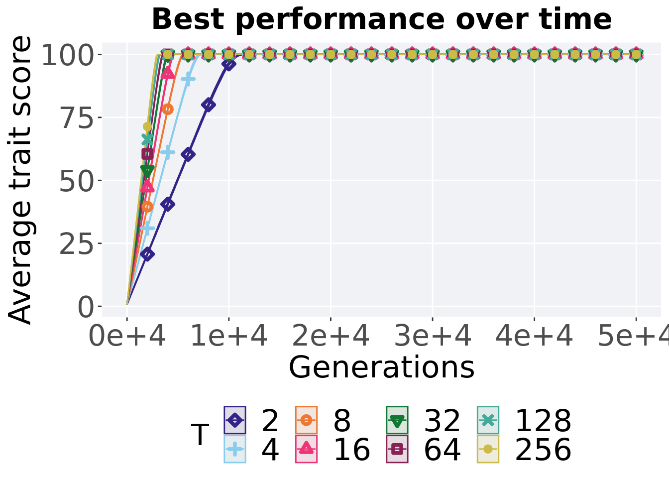

7.1.2 Generation satisfactory solution found

The first Generations a satisfactory solution is found throughout the 50,000 generations.

filter(tor_ssf, Diagnostic == 'EXPLOITATION_RATE') %>%
ggplot(., aes(x = T, y = Generations, color = T, fill = T, shape = T)) +
  geom_flat_violin(position = position_nudge(x = .2, y = 0), scale = 'width', alpha = 0.2) +
  geom_point(position = position_jitter(width = .1), size = 1.5, alpha = 1.0) +
  geom_boxplot(color = 'black', width = .2, outlier.shape = NA, alpha = 0.0) +
  scale_shape_manual(values=SHAPE)+
  scale_y_continuous(
    name="Generation",
    limits=c(0, 12000),
    breaks=c(0, 2000, 4000, 6000, 8000, 10000, 12000),
    labels=c("0e+4", "2e+4", "4e+4", "6e+4", "8e+4", "10e+4", "12e+4")
  ) +
  scale_x_discrete(
    name="T"
  ) +
  ggtitle("Generation satisfactory solution found") +
  scale_colour_manual(values = cb_palette) +
  scale_fill_manual(values = cb_palette) +
  p_theme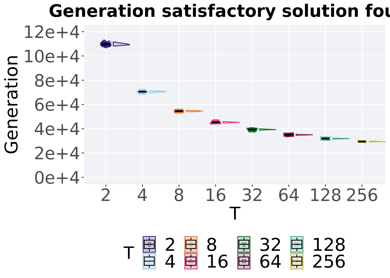

7.1.2.1 Stats

Summary statistics for the best performance found throughout 50,000 generations.

ssf = filter(tor_ssf, Diagnostic == 'EXPLOITATION_RATE')
group_by(ssf, T) %>%
  dplyr::summarise(
    count = n(),
    na_cnt = sum(is.na(Generations)),
    min = min(Generations, na.rm = TRUE),
    median = median(Generations, na.rm = TRUE),
    mean = mean(Generations, na.rm = TRUE),
    max = max(Generations, na.rm = TRUE),
    IQR = IQR(Generations, na.rm = TRUE)
  )

## # A tibble: 8 x 8
##   T     count na_cnt   min median   mean   max   IQR
##   <fct> <int>  <int> <int>  <dbl>  <dbl> <int> <dbl>
## 1 2        50      0 10815 10955  10966. 11157 102. 
## 2 4        50      0  6960  7059   7052.  7113  48.8
## 3 8        50      0  5403  5457   5453.  5519  51.8
## 4 16       50      0  4471  4530.  4532.  4597  33.8
## 5 32       50      0  3865  3938   3939.  4009  31.8
## 6 64       50      0  3446  3504.  3502.  3556  24.2
## 7 128      50      0  3152  3192   3190.  3228  26.8
## 8 256      50      0  2912  2946.  2950.  2985  24.8

Kruskal–Wallis test provides evidence of significant differences among the Generations a satisfactory solution is first found.

kruskal.test(Generations ~ T,data = ssf)

## 
##  Kruskal-Wallis rank sum test
## 
## data:  Generations by T
## Kruskal-Wallis chi-squared = 392.77, df = 7, p-value < 2.2e-16

Results for post-hoc Wilcoxon rank-sum test with a Bonferroni correction on the Generations a satisfactory solution is first found. .

pairwise.wilcox.test(x = ssf$Generations, g = ssf$T , p.adjust.method = "bonferroni",
                     paired = FALSE, conf.int = FALSE, alternative = 'l')

## 
##  Pairwise comparisons using Wilcoxon rank sum test with continuity correction 
## 
## data:  ssf$Generations and ssf$T 
## 
##     2      4      8      16     32     64     128   
## 4   <2e-16 -      -      -      -      -      -     
## 8   <2e-16 <2e-16 -      -      -      -      -     
## 16  <2e-16 <2e-16 <2e-16 -      -      -      -     
## 32  <2e-16 <2e-16 <2e-16 <2e-16 -      -      -     
## 64  <2e-16 <2e-16 <2e-16 <2e-16 <2e-16 -      -     
## 128 <2e-16 <2e-16 <2e-16 <2e-16 <2e-16 <2e-16 -     
## 256 <2e-16 <2e-16 <2e-16 <2e-16 <2e-16 <2e-16 <2e-16
## 
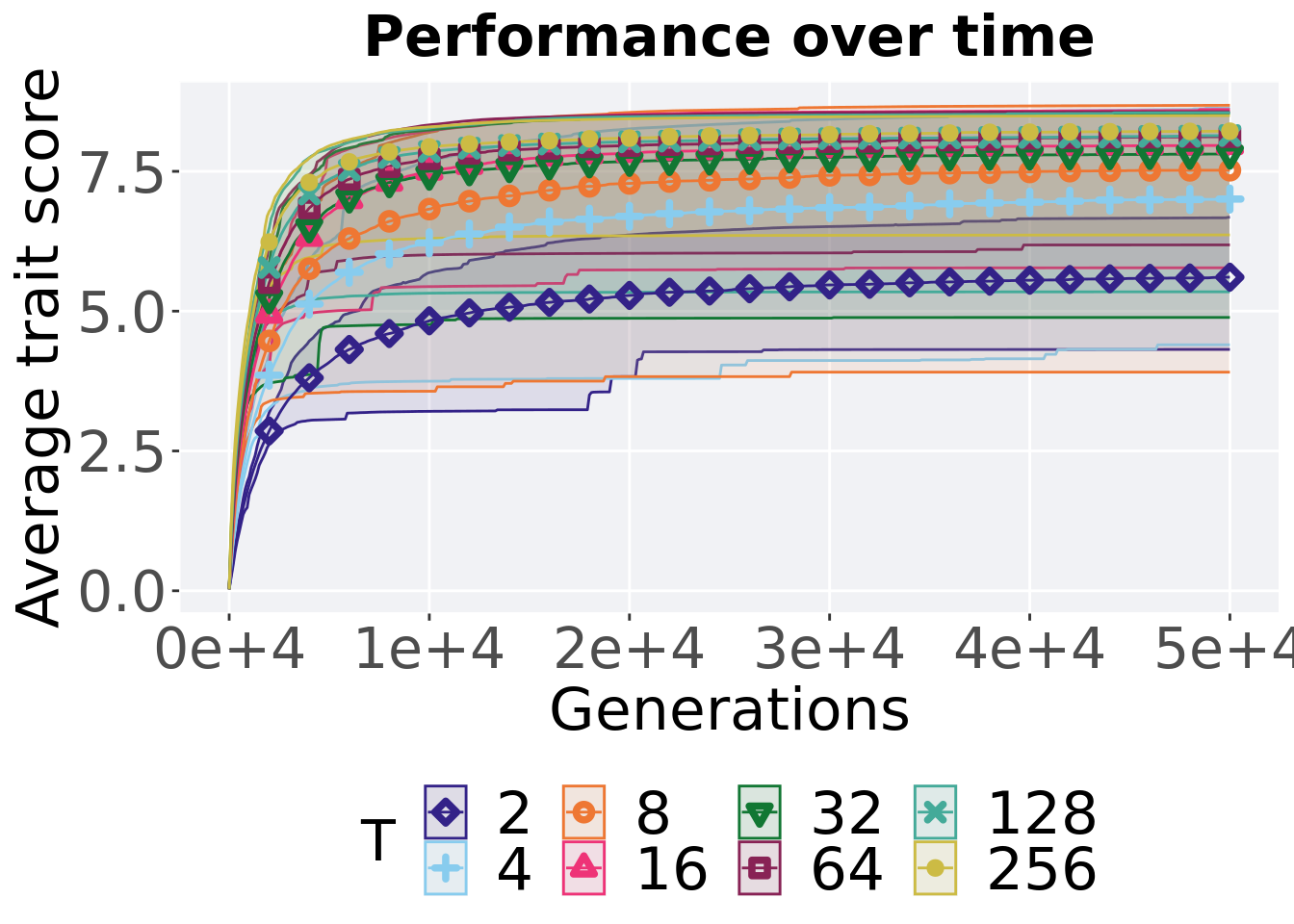
## P value adjustment method: bonferroni

7.1.3 Multi-valley crossing

7.1.3.1 Performance over time

# data for lines and shading on plots
lines = filter(tor_ot_mvc, diagnostic == 'exploitation_rate') %>%
  group_by(T, gen) %>%
  dplyr::summarise(
    min = min(pop_fit_max) / DIMENSIONALITY,
    mean = mean(pop_fit_max) / DIMENSIONALITY,
    max = max(pop_fit_max) / DIMENSIONALITY
  )

## `summarise()` has grouped output by 'T'. You can override using the `.groups`
## argument.

ggplot(lines, aes(x=gen, y=mean, group = T, fill =T, color = T, shape = T)) +
  geom_ribbon(aes(ymin = min, ymax = max), alpha = 0.1) +
  geom_line(size = 0.5) +
  geom_point(data = filter(lines, gen %% 2000 == 0 & gen != 0), size = 1.5, stroke = 2.0, alpha = 1.0) +
  scale_y_continuous(
    name="Average trait score"
  ) +
  scale_x_continuous(
    name="Generations",
    limits=c(0, 50000),
    breaks=c(0, 10000, 20000, 30000, 40000, 50000),
    labels=c("0e+4", "1e+4", "2e+4", "3e+4", "4e+4", "5e+4")

  ) +
  scale_shape_manual(values=SHAPE)+
  scale_colour_manual(values = cb_palette) +
  scale_fill_manual(values = cb_palette) +
  ggtitle('Performance over time')+
  p_theme +
  guides(
    shape=guide_legend(nrow=2, title.position = "left"),
    color=guide_legend(nrow=2, title.position = "left"),
    fill=guide_legend(nrow=2, title.position = "left")
  )

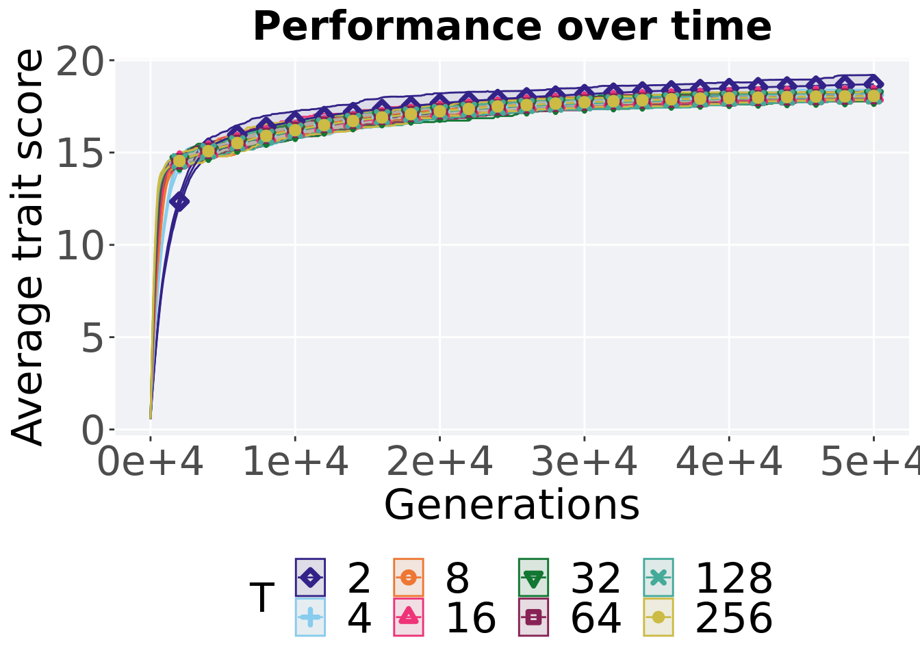
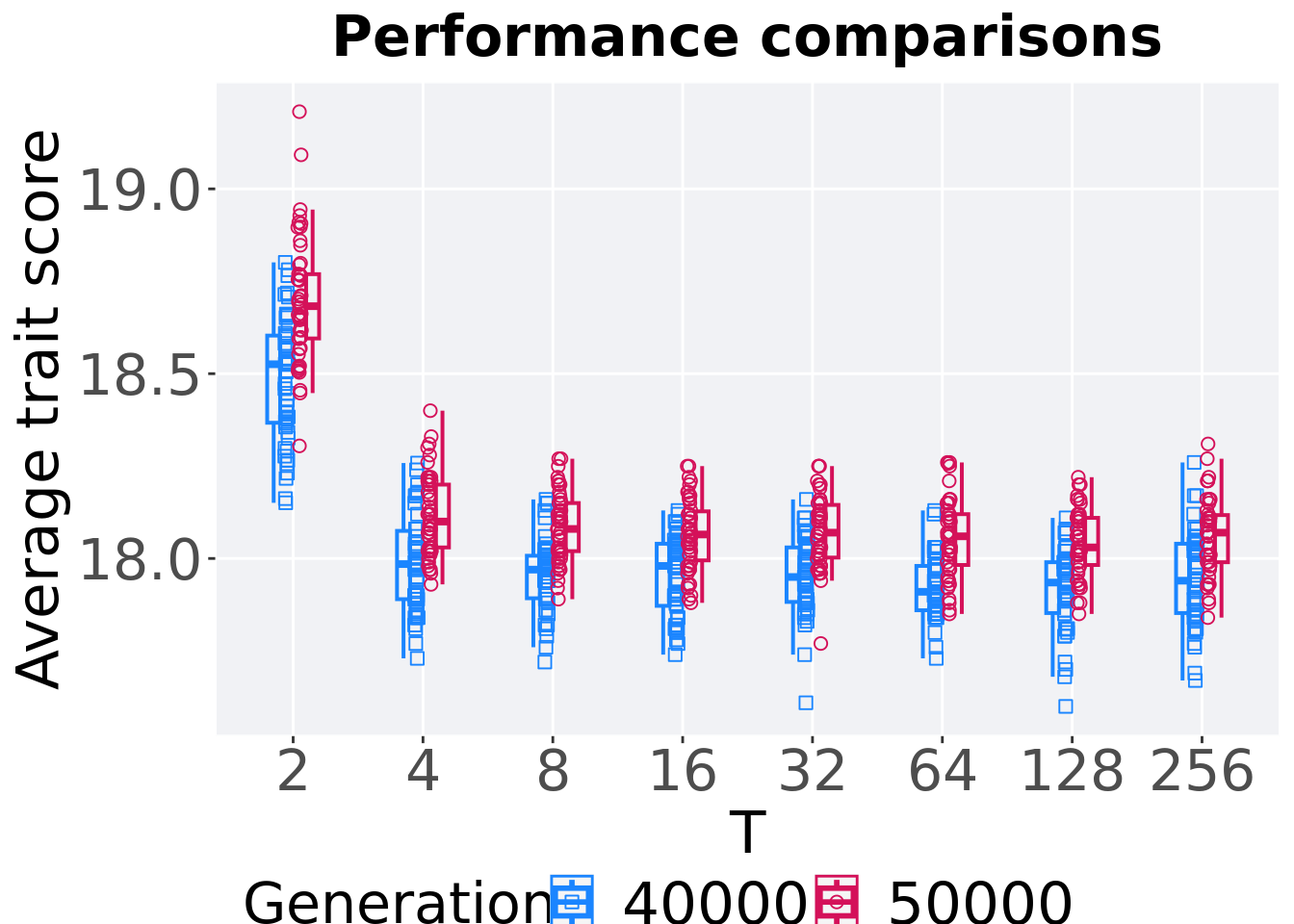
7.1.3.2 Performance comparison

Best performances in the population at 40,000 and 50,000 generations.

# 80% and final generation comparison
end = filter(tor_ot_mvc, diagnostic == 'exploitation_rate' & gen == 50000 & T != 'ran')
end$Generation <- factor(end$gen)

mid = filter(tor_ot_mvc, diagnostic == 'exploitation_rate' & gen == 40000 & T != 'ran')
mid$Generation <- factor(mid$gen)

mvc_p = ggplot(mid, aes(x = T, y=pop_fit_max / DIMENSIONALITY, group = T, shape = Generation)) +
  geom_point(col = mvc_col[1] , position = position_jitternudge(jitter.width = .03, nudge.x = -0.05), size = 2, alpha = 1.0) +
  geom_boxplot(position = position_nudge(x = -.15, y = 0), lwd = 0.7, col = mvc_col[1], fill = mvc_col[1], width = .1, outlier.shape = NA, alpha = 0.0) +

  geom_point(data = end, aes(x = T, y=pop_fit_max / DIMENSIONALITY), col = mvc_col[2], position = position_jitternudge(jitter.width = .03, nudge.x = 0.05), size = 2, alpha = 1.0) +
  geom_boxplot(data = end, aes(x = T, y=pop_fit_max / DIMENSIONALITY), position = position_nudge(x = .15, y = 0), lwd = 0.7, col = mvc_col[2], fill = mvc_col[2], width = .1, outlier.shape = NA, alpha = 0.0) +

  scale_y_continuous(
    name="Average trait score"
  ) +
  scale_x_discrete(
    name="T"
  )+
  scale_shape_manual(values=c(0,1))+
  scale_colour_manual(values = c(mvc_col[1],mvc_col[2])) +
  p_theme

plot_grid(
  mvc_p +
    ggtitle("Performance comparisons") +
    theme(legend.position="none"),
  legend,
  nrow=2,
  rel_heights = c(1,.05),
  label_size = TSIZE
)

7.1.3.3 Stats

Summary statistics for the performance of the best performance at 40,000 and 50,000 generations.

slices = filter(tor_ot_mvc, diagnostic == 'exploitation_rate' & (gen == 50000 | gen == 40000))
slices$Generation <- factor(slices$gen, levels = c(50000,40000))
slices %>%
  group_by(T, Generation) %>%
  dplyr::summarise(
    count = n(),
    na_cnt = sum(is.na(pop_fit_max  / DIMENSIONALITY)),
    min = min(pop_fit_max  / DIMENSIONALITY, na.rm = TRUE),
    median = median(pop_fit_max  / DIMENSIONALITY, na.rm = TRUE),
    mean = mean(pop_fit_max  / DIMENSIONALITY, na.rm = TRUE),
    max = max(pop_fit_max  / DIMENSIONALITY, na.rm = TRUE),
    IQR = IQR(pop_fit_max  / DIMENSIONALITY, na.rm = TRUE)
  )

## `summarise()` has grouped output by 'T'. You can override using the `.groups`
## argument.

## # A tibble: 16 x 9
## # Groups:   T [8]
##    T     Generation count na_cnt   min median  mean   max   IQR
##    <fct> <fct>      <int>  <int> <dbl>  <dbl> <dbl> <dbl> <dbl>
##  1 2     50000         50      0  18.3   18.7  18.7  19.2 0.174
##  2 2     40000         50      0  18.2   18.5  18.5  18.8 0.236
##  3 4     50000         50      0  17.9   18.1  18.1  18.4 0.170
##  4 4     40000         50      0  17.7   18.0  18.0  18.3 0.185
##  5 8     50000         50      0  17.9   18.1  18.1  18.3 0.130
##  6 8     40000         50      0  17.7   18.0  18.0  18.2 0.115
##  7 16    50000         50      0  17.9   18.1  18.1  18.2 0.133
##  8 16    40000         50      0  17.7   18.0  18.0  18.1 0.168
##  9 32    50000         50      0  17.8   18.1  18.1  18.2 0.142
## 10 32    40000         50      0  17.6   17.9  18.0  18.2 0.147
## 11 64    50000         50      0  17.8   18.1  18.1  18.3 0.137
## 12 64    40000         50      0  17.7   17.9  17.9  18.1 0.120
## 13 128   50000         50      0  17.8   18.0  18.0  18.2 0.128
## 14 128   40000         50      0  17.6   17.9  17.9  18.1 0.137
## 15 256   50000         50      0  17.8   18.1  18.1  18.3 0.128
## 16 256   40000         50      0  17.7   17.9  18.0  18.3 0.188

T 2

wilcox.test(x = filter(slices, T == 2 & Generation == 50000)$pop_fit_max,
            y = filter(slices, T == 2 & Generation == 40000)$pop_fit_max,
            alternative = 't')

## 
##  Wilcoxon rank sum test with continuity correction
## 
## data:  filter(slices, T == 2 & Generation == 50000)$pop_fit_max and filter(slices, T == 2 & Generation == 40000)$pop_fit_max
## W = 2007, p-value = 1.836e-07
## alternative hypothesis: true location shift is not equal to 0

T 4

wilcox.test(x = filter(slices, T == 4 & Generation == 50000)$pop_fit_max,
            y = filter(slices, T == 4 & Generation == 40000)$pop_fit_max,
            alternative = 't')

## 
##  Wilcoxon rank sum test with continuity correction
## 
## data:  filter(slices, T == 4 & Generation == 50000)$pop_fit_max and filter(slices, T == 4 & Generation == 40000)$pop_fit_max
## W = 1961, p-value = 9.59e-07
## alternative hypothesis: true location shift is not equal to 0

T 8

wilcox.test(x = filter(slices, T == 8 & Generation == 50000)$pop_fit_max,
            y = filter(slices, T == 8 & Generation == 40000)$pop_fit_max,
            alternative = 't')

## 
##  Wilcoxon rank sum test with continuity correction
## 
## data:  filter(slices, T == 8 & Generation == 50000)$pop_fit_max and filter(slices, T == 8 & Generation == 40000)$pop_fit_max
## W = 2075, p-value = 1.301e-08
## alternative hypothesis: true location shift is not equal to 0

T 16

wilcox.test(x = filter(slices, T == 16 & Generation == 50000)$pop_fit_max,
            y = filter(slices, T == 16 & Generation == 40000)$pop_fit_max,
            alternative = 't')

## 
##  Wilcoxon rank sum test with continuity correction
## 
## data:  filter(slices, T == 16 & Generation == 50000)$pop_fit_max and filter(slices, T == 16 & Generation == 40000)$pop_fit_max
## W = 1948.5, p-value = 1.483e-06
## alternative hypothesis: true location shift is not equal to 0

T 32

wilcox.test(x = filter(slices, T == 32 & Generation == 50000)$pop_fit_max,
            y = filter(slices, T == 32 & Generation == 40000)$pop_fit_max,
            alternative = 't')

## 
##  Wilcoxon rank sum test with continuity correction
## 
## data:  filter(slices, T == 32 & Generation == 50000)$pop_fit_max and filter(slices, T == 32 & Generation == 40000)$pop_fit_max
## W = 2020.5, p-value = 1.097e-07
## alternative hypothesis: true location shift is not equal to 0

T 64

wilcox.test(x = filter(slices, T == 64 & Generation == 50000)$pop_fit_max,
            y = filter(slices, T == 64 & Generation == 40000)$pop_fit_max,
            alternative = 't')

## 
##  Wilcoxon rank sum test with continuity correction
## 
## data:  filter(slices, T == 64 & Generation == 50000)$pop_fit_max and filter(slices, T == 64 & Generation == 40000)$pop_fit_max
## W = 2104.5, p-value = 3.84e-09
## alternative hypothesis: true location shift is not equal to 0

T 128

wilcox.test(x = filter(slices, T == 128 & Generation == 50000)$pop_fit_max,
            y = filter(slices, T == 128 & Generation == 40000)$pop_fit_max,
            alternative = 't')

## 
##  Wilcoxon rank sum test with continuity correction
## 
## data:  filter(slices, T == 128 & Generation == 50000)$pop_fit_max and filter(slices, T == 128 & Generation == 40000)$pop_fit_max
## W = 2003.5, p-value = 2.068e-07
## alternative hypothesis: true location shift is not equal to 0

T 256

wilcox.test(x = filter(slices, T == 256 & Generation == 50000)$pop_fit_max,
            y = filter(slices, T == 256 & Generation == 40000)$pop_fit_max,
            alternative = 't')

## 
##  Wilcoxon rank sum test with continuity correction
## 
## data:  filter(slices, T == 256 & Generation == 50000)$pop_fit_max and filter(slices, T == 256 & Generation == 40000)$pop_fit_max
## W = 1892.5, p-value = 9.536e-06
## alternative hypothesis: true location shift is not equal to 0

7.2 Ordered exploitation results

Here we present the results for best performances found by each tournament selection size value replicate on the ordered exploitation diagnostic. Best performance found refers to the largest average trait score found in a given population. Note that performance values fall between 0 and 100.

7.2.1 Performance over time

Performance over time.

lines = filter(tor_ot, diagnostic == 'ordered_exploitation') %>%
        group_by(T, gen) %>%
          dplyr::summarise(
            min = min(pop_fit_max),
            mean = mean(pop_fit_max),
            max = max(pop_fit_max)
          )

## `summarise()` has grouped output by 'T'. You can override using the `.groups`
## argument.

ggplot(lines, aes(x=gen, y=mean / DIMENSIONALITY, group = T, fill = T, color = T, shape = T)) +
  geom_ribbon(aes(ymin = min / DIMENSIONALITY, ymax = max / DIMENSIONALITY), alpha = 0.1) +
  geom_line(size = 0.5) +
  geom_point(data = filter(lines, gen %% 2000 == 0 & gen != 0), size = 1.5, stroke = 2.0, alpha = 1.0) +
  scale_y_continuous(
    name="Average trait score",
    limits=c(-1, 101),
    breaks=seq(0,100, 20),
    labels=c("0", "20", "40", "60", "80", "100")
  ) +
  scale_x_continuous(
    name="Generations",
    limits=c(0, 50000),
    breaks=c(0, 10000, 20000, 30000, 40000, 50000),
    labels=c("0e+4", "1e+4", "2e+4", "3e+4", "4e+4", "5e+4")

  ) +
  scale_shape_manual(values=SHAPE)+
  scale_colour_manual(values = cb_palette) +
  scale_fill_manual(values = cb_palette) +
  ggtitle("Best performance over time") +
  p_theme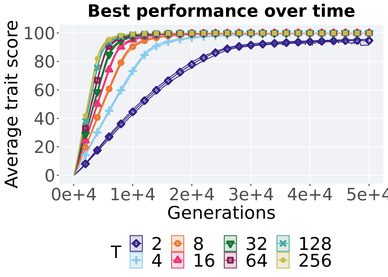

7.2.2 Generation satisfactory solution found

The first Generations a satisfactory solution is found throughout the 50,000 generations.

filter(tor_ssf, Diagnostic == 'ORDERED_EXPLOITATION') %>%
ggplot(., aes(x = T, y = Generations, color = T, fill = T, shape = T)) +
  geom_flat_violin(position = position_nudge(x = .2, y = 0), scale = 'width', alpha = 0.2) +
  geom_point(position = position_jitter(width = .1), size = 1.5, alpha = 1.0) +
  geom_boxplot(color = 'black', width = .2, outlier.shape = NA, alpha = 0.0) +
  scale_shape_manual(values=SHAPE)+
  scale_y_continuous(
    name="Generation",
    limits=c(0, 60000),
    breaks=c(0, 10000, 20000, 30000, 40000, 50000, 60000),
    labels=c("0e+4", "1e+4", "2e+4", "3e+4", "4e+4", "5e+4", "Fail")
  ) +
  scale_x_discrete(
    name="T"
  ) +
  scale_colour_manual(values = cb_palette) +
  scale_fill_manual(values = cb_palette) +
  ggtitle("Generation satisfactory solution found") +
  p_theme

## Warning: Removed 15 rows containing missing values (`geom_point()`).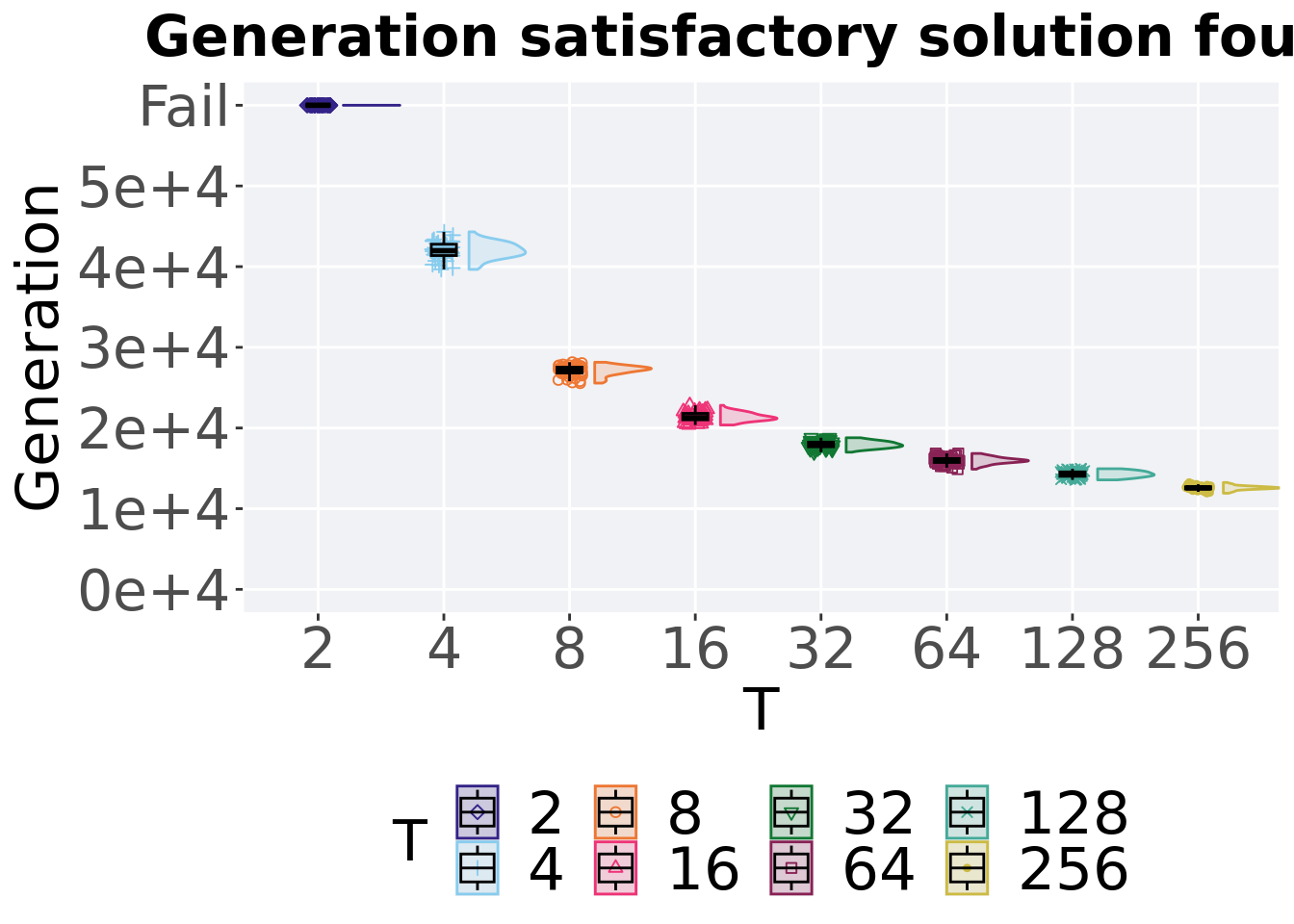

7.2.2.1 Stats

Summary statistics for the first Generations a satisfactory solution is found throughout the 50,000 generations.

ssf = filter(tor_ssf, Diagnostic == 'ORDERED_EXPLOITATION')
group_by(ssf, T) %>%
  dplyr::summarise(
    count = n(),
    na_cnt = sum(is.na(Generations)),
    min = min(Generations, na.rm = TRUE),
    median = median(Generations, na.rm = TRUE),
    mean = mean(Generations, na.rm = TRUE),
    max = max(Generations, na.rm = TRUE),
    IQR = IQR(Generations, na.rm = TRUE)
  )

## # A tibble: 8 x 8
##   T     count na_cnt   min median   mean   max   IQR
##   <fct> <int>  <int> <int>  <dbl>  <dbl> <int> <dbl>
## 1 2        50      0 60000 60000  60000  60000    0 
## 2 4        50      0 39659 41972. 41991. 44310 1404.
## 3 8        50      0 25563 27254. 27122. 28151  714 
## 4 16       50      0 20374 21270. 21366. 22808  792.
## 5 32       50      0 17005 17945  17950. 18792  572.
## 6 64       50      0 14896 15960  15965. 16845  480.
## 7 128      50      0 13569 14278. 14278. 14952  545 
## 8 256      50      0 11919 12578. 12580. 13249  262.

Kruskal–Wallis test provides evidence of significant differences among the first Generations a satisfactory solution is found throughout the 50,000 generations.

kruskal.test(Generations ~ T, data = ssf)

## 
##  Kruskal-Wallis rank sum test
## 
## data:  Generations by T
## Kruskal-Wallis chi-squared = 393.52, df = 7, p-value < 2.2e-16

Results for post-hoc Wilcoxon rank-sum test with a Bonferroni correction on the first Generations a satisfactory solution is found throughout the 50,000 generations.

pairwise.wilcox.test(x = ssf$Generations, g = ssf$T , p.adjust.method = "bonferroni",
                     paired = FALSE, conf.int = FALSE, alternative = 'l')

## 
##  Pairwise comparisons using Wilcoxon rank sum test with continuity correction 
## 
## data:  ssf$Generations and ssf$T 
## 
##     2      4      8      16     32     64     128   
## 4   <2e-16 -      -      -      -      -      -     
## 8   <2e-16 <2e-16 -      -      -      -      -     
## 16  <2e-16 <2e-16 <2e-16 -      -      -      -     
## 32  <2e-16 <2e-16 <2e-16 <2e-16 -      -      -     
## 64  <2e-16 <2e-16 <2e-16 <2e-16 <2e-16 -      -     
## 128 <2e-16 <2e-16 <2e-16 <2e-16 <2e-16 <2e-16 -     
## 256 <2e-16 <2e-16 <2e-16 <2e-16 <2e-16 <2e-16 <2e-16
## 
## P value adjustment method: bonferroni

7.2.3 Multi-valley crossing

7.2.3.1 Performance over time

# data for lines and shading on plots
lines = filter(tor_ot_mvc, diagnostic == 'ordered_exploitation') %>%
  group_by(T, gen) %>%
  dplyr::summarise(
    min = min(pop_fit_max) / DIMENSIONALITY,
    mean = mean(pop_fit_max) / DIMENSIONALITY,
    max = max(pop_fit_max) / DIMENSIONALITY
  )

## `summarise()` has grouped output by 'T'. You can override using the `.groups`
## argument.

ggplot(lines, aes(x=gen, y=mean, group = T, fill =T, color = T, shape = T)) +
  geom_ribbon(aes(ymin = min, ymax = max), alpha = 0.1) +
  geom_line(size = 0.5) +
  geom_point(data = filter(lines, gen %% 2000 == 0 & gen != 0), size = 1.5, stroke = 2.0, alpha = 1.0) +
  scale_y_continuous(
    name="Average trait score"
  ) +
  scale_x_continuous(
    name="Generations",
    limits=c(0, 50000),
    breaks=c(0, 10000, 20000, 30000, 40000, 50000),
    labels=c("0e+4", "1e+4", "2e+4", "3e+4", "4e+4", "5e+4")

  ) +
  scale_shape_manual(values=SHAPE)+
  scale_colour_manual(values = cb_palette) +
  scale_fill_manual(values = cb_palette) +
  ggtitle('Performance over time')+
  p_theme +
  guides(
    shape=guide_legend(nrow=2, title.position = "left"),
    color=guide_legend(nrow=2, title.position = "left"),
    fill=guide_legend(nrow=2, title.position = "left")
  )

7.2.3.2 Performance comparison

Best performances in the population at 40,000 and 50,000 generations.

# 80% and final generation comparison
end = filter(tor_ot_mvc, diagnostic == 'ordered_exploitation' & gen == 50000 & T != 'ran')
end$Generation <- factor(end$gen)

mid = filter(tor_ot_mvc, diagnostic == 'ordered_exploitation' & gen == 40000 & T != 'ran')
mid$Generation <- factor(mid$gen)

mvc_p = ggplot(mid, aes(x = T, y=pop_fit_max / DIMENSIONALITY, group = T, shape = Generation)) +
  geom_point(col = mvc_col[1] , position = position_jitternudge(jitter.width = .03, nudge.x = -0.05), size = 2, alpha = 1.0) +
  geom_boxplot(position = position_nudge(x = -.15, y = 0), lwd = 0.7, col = mvc_col[1], fill = mvc_col[1], width = .1, outlier.shape = NA, alpha = 0.0) +

  geom_point(data = end, aes(x = T, y=pop_fit_max / DIMENSIONALITY), col = mvc_col[2], position = position_jitternudge(jitter.width = .03, nudge.x = 0.05), size = 2, alpha = 1.0) +
  geom_boxplot(data = end, aes(x = T, y=pop_fit_max / DIMENSIONALITY), position = position_nudge(x = .15, y = 0), lwd = 0.7, col = mvc_col[2], fill = mvc_col[2], width = .1, outlier.shape = NA, alpha = 0.0) +

  scale_y_continuous(
    name="Average trait score"
  ) +
  scale_x_discrete(
    name="T"
  )+
  scale_shape_manual(values=c(0,1))+
  scale_colour_manual(values = c(mvc_col[1],mvc_col[2])) +
  p_theme

plot_grid(
  mvc_p +
    ggtitle("Performance comparisons") +
    theme(legend.position="none"),
  legend,
  nrow=2,
  rel_heights = c(1,.05),
  label_size = TSIZE
)

7.2.3.3 Stats

Summary statistics for the performance of the best performance at 40,000 and 50,000 generations.

slices = filter(tor_ot_mvc, diagnostic == 'ordered_exploitation' & (gen == 50000 | gen == 40000))
slices$Generation <- factor(slices$gen, levels = c(50000,40000))
slices %>%
  group_by(T, Generation) %>%
  dplyr::summarise(
    count = n(),
    na_cnt = sum(is.na(pop_fit_max  / DIMENSIONALITY)),
    min = min(pop_fit_max  / DIMENSIONALITY, na.rm = TRUE),
    median = median(pop_fit_max  / DIMENSIONALITY, na.rm = TRUE),
    mean = mean(pop_fit_max  / DIMENSIONALITY, na.rm = TRUE),
    max = max(pop_fit_max  / DIMENSIONALITY, na.rm = TRUE),
    IQR = IQR(pop_fit_max  / DIMENSIONALITY, na.rm = TRUE)
  )

## `summarise()` has grouped output by 'T'. You can override using the `.groups`
## argument.

## # A tibble: 16 x 9
## # Groups:   T [8]
##    T     Generation count na_cnt   min median  mean   max   IQR
##    <fct> <fct>      <int>  <int> <dbl>  <dbl> <dbl> <dbl> <dbl>
##  1 2     50000         50      0  4.32   5.73  5.61  6.68 0.858
##  2 2     40000         50      0  4.31   5.64  5.55  6.65 0.835
##  3 4     50000         50      0  4.40   7.24  7.00  8.64 1.41 
##  4 4     40000         50      0  4.15   7.22  6.95  8.54 1.43 
##  5 8     50000         50      0  3.91   7.76  7.52  8.68 1.26 
##  6 8     40000         50      0  3.91   7.74  7.49  8.67 1.24 
##  7 16    50000         50      0  5.78   8.33  7.96  8.61 0.905
##  8 16    40000         50      0  5.77   8.31  7.95  8.58 0.903
##  9 32    50000         50      0  4.89   8.28  7.81  8.54 0.952
## 10 32    40000         50      0  4.89   8.26  7.79  8.53 0.950
## 11 64    50000         50      0  6.18   8.34  8.12  8.57 0.273
## 12 64    40000         50      0  6.18   8.31  8.09  8.56 0.316
## 13 128   50000         50      0  5.35   8.34  8.14  8.55 0.112
## 14 128   40000         50      0  5.34   8.31  8.11  8.53 0.132
## 15 256   50000         50      0  6.36   8.35  8.22  8.50 0.128
## 16 256   40000         50      0  6.36   8.34  8.20  8.49 0.119

T 2

wilcox.test(x = filter(slices, T == 2 & Generation == 50000)$pop_fit_max,
            y = filter(slices, T == 2 & Generation == 40000)$pop_fit_max,
            alternative = 't')

## 
##  Wilcoxon rank sum test with continuity correction
## 
## data:  filter(slices, T == 2 & Generation == 50000)$pop_fit_max and filter(slices, T == 2 & Generation == 40000)$pop_fit_max
## W = 1337, p-value = 0.551
## alternative hypothesis: true location shift is not equal to 0

T 4

wilcox.test(x = filter(slices, T == 4 & Generation == 50000)$pop_fit_max,
            y = filter(slices, T == 4 & Generation == 40000)$pop_fit_max,
            alternative = 't')

## 
##  Wilcoxon rank sum test with continuity correction
## 
## data:  filter(slices, T == 4 & Generation == 50000)$pop_fit_max and filter(slices, T == 4 & Generation == 40000)$pop_fit_max
## W = 1315, p-value = 0.6566
## alternative hypothesis: true location shift is not equal to 0

T 8

wilcox.test(x = filter(slices, T == 8 & Generation == 50000)$pop_fit_max,
            y = filter(slices, T == 8 & Generation == 40000)$pop_fit_max,
            alternative = 't')

## 
##  Wilcoxon rank sum test with continuity correction
## 
## data:  filter(slices, T == 8 & Generation == 50000)$pop_fit_max and filter(slices, T == 8 & Generation == 40000)$pop_fit_max
## W = 1306.5, p-value = 0.6995
## alternative hypothesis: true location shift is not equal to 0

T 16

wilcox.test(x = filter(slices, T == 16 & Generation == 50000)$pop_fit_max,
            y = filter(slices, T == 16 & Generation == 40000)$pop_fit_max,
            alternative = 't')

## 
##  Wilcoxon rank sum test with continuity correction
## 
## data:  filter(slices, T == 16 & Generation == 50000)$pop_fit_max and filter(slices, T == 16 & Generation == 40000)$pop_fit_max
## W = 1309, p-value = 0.6867
## alternative hypothesis: true location shift is not equal to 0

T 32

wilcox.test(x = filter(slices, T == 32 & Generation == 50000)$pop_fit_max,
            y = filter(slices, T == 32 & Generation == 40000)$pop_fit_max,
            alternative = 't')

## 
##  Wilcoxon rank sum test with continuity correction
## 
## data:  filter(slices, T == 32 & Generation == 50000)$pop_fit_max and filter(slices, T == 32 & Generation == 40000)$pop_fit_max
## W = 1305, p-value = 0.7071
## alternative hypothesis: true location shift is not equal to 0

T 64

wilcox.test(x = filter(slices, T == 64 & Generation == 50000)$pop_fit_max,
            y = filter(slices, T == 64 & Generation == 40000)$pop_fit_max,
            alternative = 't')

## 
##  Wilcoxon rank sum test with continuity correction
## 
## data:  filter(slices, T == 64 & Generation == 50000)$pop_fit_max and filter(slices, T == 64 & Generation == 40000)$pop_fit_max
## W = 1379, p-value = 0.3757
## alternative hypothesis: true location shift is not equal to 0

T 128

wilcox.test(x = filter(slices, T == 128 & Generation == 50000)$pop_fit_max,
            y = filter(slices, T == 128 & Generation == 40000)$pop_fit_max,
            alternative = 't')

## 
##  Wilcoxon rank sum test with continuity correction
## 
## data:  filter(slices, T == 128 & Generation == 50000)$pop_fit_max and filter(slices, T == 128 & Generation == 40000)$pop_fit_max
## W = 1409, p-value = 0.2745
## alternative hypothesis: true location shift is not equal to 0

T 256

wilcox.test(x = filter(slices, T == 256 & Generation == 50000)$pop_fit_max,
            y = filter(slices, T == 256 & Generation == 40000)$pop_fit_max,
            alternative = 't')

## 
##  Wilcoxon rank sum test with continuity correction
## 
## data:  filter(slices, T == 256 & Generation == 50000)$pop_fit_max and filter(slices, T == 256 & Generation == 40000)$pop_fit_max
## W = 1381, p-value = 0.3683
## alternative hypothesis: true location shift is not equal to 0

7.3 Contraditory objectives diagnostic

Here we present the results for satisfactory trait coverage and activation gene coverage found by each tournament selection size value replicate on the ordered exploitation diagnostic. Satisfactory trait coverage refers to the count of unique satisfied traits in the population, while activation gene coverage refers to the count of unique activation genes in the population. Note that both coverage values fall between 0 and 100.

7.3.1 Satisfactory trait coverage

Satisfactory trait coverage analysis.

7.3.1.1 Coverage over time

Satisfactory trait coverage over time.

lines = filter(tor_ot, diagnostic == 'contradictory_objectives') %>%
        group_by(T, gen) %>%
          dplyr::summarise(
            min = min(pop_uni_obj),
            mean = mean(pop_uni_obj),
            max = max(pop_uni_obj)
          )

## `summarise()` has grouped output by 'T'. You can override using the `.groups`
## argument.

ggplot(lines, aes(x=gen, y=mean, group = T, fill =T, color = T, shape = T)) +
  geom_ribbon(aes(ymin = min, ymax = max), alpha = 0.1) +
  geom_line(size = 0.5) +
  geom_point(data = filter(lines, gen %% 2000 == 0 & gen != 0), size = 1.5, stroke = 2.0, alpha = 1.0) +
  scale_y_continuous(
    name="Coverage"
  ) +
  scale_x_continuous(
    name="Generations",
    limits=c(0, 50000),
    breaks=c(0, 10000, 20000, 30000, 40000, 50000),
    labels=c("0e+4", "1e+4", "2e+4", "3e+4", "4e+4", "5e+4")

  ) +
  scale_shape_manual(values=SHAPE)+
  scale_colour_manual(values = cb_palette) +
  scale_fill_manual(values = cb_palette) +
  ggtitle("Satisfactory trait coverage over time") +
  p_theme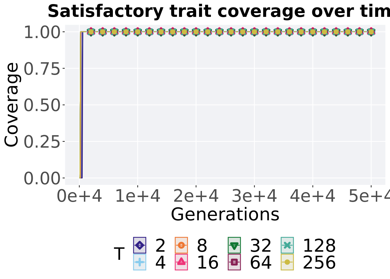

7.3.1.2 Best coverage throughout

Best satisfactory trait coverage throughout 50,000 generations.

filter(tor_best, col == 'pop_uni_obj' & diagnostic == 'contradictory_objectives') %>%
ggplot(., aes(x = T, y = val, color = T, fill = T, shape = T)) +
  geom_flat_violin(position = position_nudge(x = .2, y = 0), scale = 'width', alpha = 0.2) +
  geom_point(position = position_jitter(width = .1), size = 1.5, alpha = 1.0) +
  geom_boxplot(color = 'black', width = .2, outlier.shape = NA, alpha = 0.0) +
  scale_y_continuous(
    name="Coverage"
  ) +
  scale_x_discrete(
    name="T"
  )+
  scale_shape_manual(values=SHAPE)+
  scale_colour_manual(values = cb_palette) +
  scale_fill_manual(values = cb_palette) +
  ggtitle("Best satisfactory trait coverage") +
  p_theme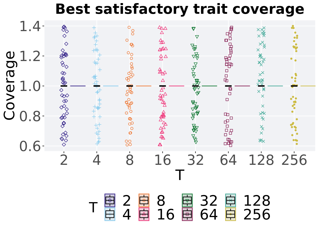

7.3.1.2.1 Stats

Summary statistics for the best satisfactory trait coverage throughout 50,000 generations.

coverage = filter(tor_best, col == 'pop_uni_obj' & diagnostic == 'contradictory_objectives')
group_by(coverage, T) %>%
  dplyr::summarise(
    count = n(),
    na_cnt = sum(is.na(val)),
    min = min(val, na.rm = TRUE),
    median = median(val, na.rm = TRUE),
    mean = mean(val, na.rm = TRUE),
    max = max(val, na.rm = TRUE),
    IQR = IQR(val, na.rm = TRUE)
  )

## # A tibble: 8 x 8
##   T     count na_cnt   min median  mean   max   IQR
##   <fct> <int>  <int> <dbl>  <dbl> <dbl> <dbl> <dbl>
## 1 2        50      0     1      1     1     1     0
## 2 4        50      0     1      1     1     1     0
## 3 8        50      0     1      1     1     1     0
## 4 16       50      0     1      1     1     1     0
## 5 32       50      0     1      1     1     1     0
## 6 64       50      0     1      1     1     1     0
## 7 128      50      0     1      1     1     1     0
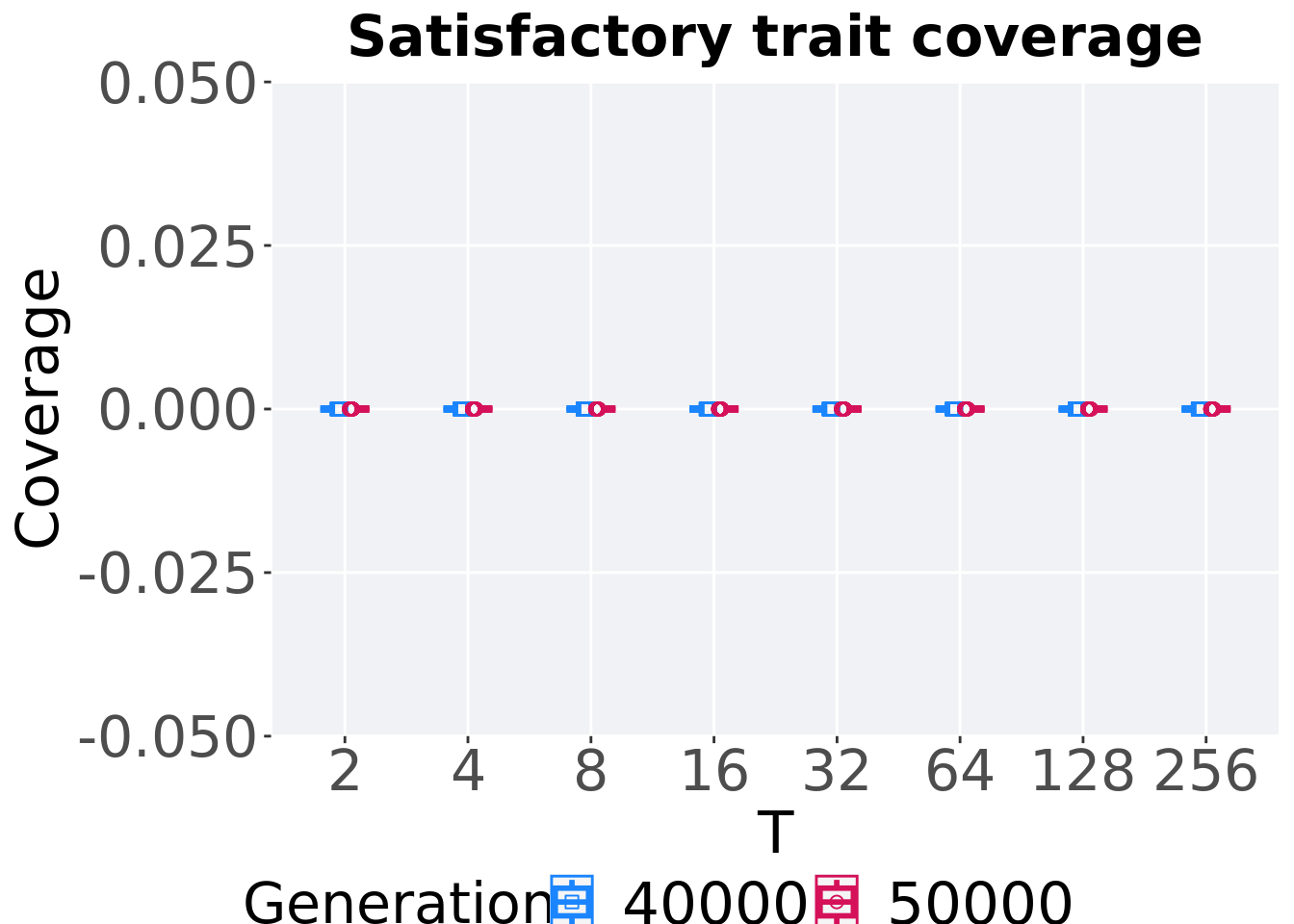
## 8 256      50      0     1      1     1     1     0

7.3.1.3 End of 50,000 generations

Satisfactory trait coverage in the population at the end of 50,000 generations.

filter(tor_ot, diagnostic == 'contradictory_objectives' & gen == 50000) %>%
ggplot(., aes(x = T, y = pop_uni_obj, color = T, fill = T, shape = T)) +
  geom_flat_violin(position = position_nudge(x = .2, y = 0), scale = 'width', alpha = 0.2) +
  geom_point(position = position_jitter(width = .1), size = 1.5, alpha = 1.0) +
  geom_boxplot(color = 'black', width = .2, outlier.shape = NA, alpha = 0.0) +
  scale_y_continuous(
    name="Coverage"
  ) +
  scale_x_discrete(
    name="T"
  )+
  scale_shape_manual(values=SHAPE)+
  scale_colour_manual(values = cb_palette) +
  scale_fill_manual(values = cb_palette) +
  ggtitle("Final satisfactory trait coverage") +
  p_theme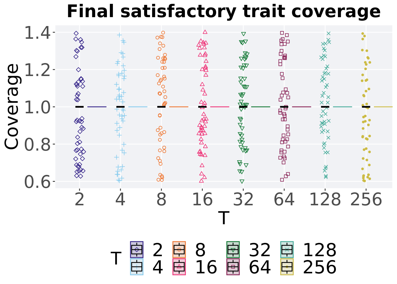

7.3.1.3.1 Stats

Summary statistics for satisfactory trait coverage in the population at the end of 50,000 generations.

coverage = filter(tor_ot, diagnostic == 'contradictory_objectives' & gen == 50000)
group_by(coverage, T) %>%
  dplyr::summarise(
    count = n(),
    na_cnt = sum(is.na(pop_uni_obj)),
    min = min(pop_uni_obj, na.rm = TRUE),
    median = median(pop_uni_obj, na.rm = TRUE),
    mean = mean(pop_uni_obj, na.rm = TRUE),
    max = max(pop_uni_obj, na.rm = TRUE),
    IQR = IQR(pop_uni_obj, na.rm = TRUE)
  )

## # A tibble: 8 x 8
##   T     count na_cnt   min median  mean   max   IQR
##   <fct> <int>  <int> <int>  <dbl> <dbl> <int> <dbl>
## 1 2        50      0     1      1     1     1     0
## 2 4        50      0     1      1     1     1     0
## 3 8        50      0     1      1     1     1     0
## 4 16       50      0     1      1     1     1     0
## 5 32       50      0     1      1     1     1     0
## 6 64       50      0     1      1     1     1     0
## 7 128      50      0     1      1     1     1     0
## 8 256      50      0     1      1     1     1     0

7.3.2 Activation gene coverage

Here we analyze the activation gene coverage for each parameter replicate on the contradictory objectives diagnostic.

7.3.2.1 Coverage over time

Activation gene coverage over time.

lines = filter(tor_ot, diagnostic == 'contradictory_objectives') %>%
        group_by(T, gen) %>%
          dplyr::summarise(
            min = min(uni_str_pos),
            mean = mean(uni_str_pos),
            max = max(uni_str_pos)
          )

## `summarise()` has grouped output by 'T'. You can override using the `.groups`
## argument.

ggplot(lines, aes(x=gen, y=mean, group = T, fill =T, color = T, shape = T)) +
  geom_ribbon(aes(ymin = min, ymax = max), alpha = 0.1) +
  geom_line(size = 0.5) +
  geom_point(data = filter(lines, gen %% 2000 == 0 & gen != 0), size = 1.5, stroke = 2.0, alpha = 1.0) +
  scale_y_continuous(
    name="Coverage",
    limits=c(-1, 101),
    breaks=seq(0,100, 20),
    labels=c("0", "20", "40", "60", "80", "100")
  ) +
  scale_x_continuous(
    name="Generations",
    limits=c(0, 50000),
    breaks=c(0, 10000, 20000, 30000, 40000, 50000),
    labels=c("0e+4", "1e+4", "2e+4", "3e+4", "4e+4", "5e+4")

  ) +
  scale_shape_manual(values=SHAPE)+
  scale_colour_manual(values = cb_palette) +
  scale_fill_manual(values = cb_palette) +
  ggtitle("Activation gene coverage over time") +
  p_theme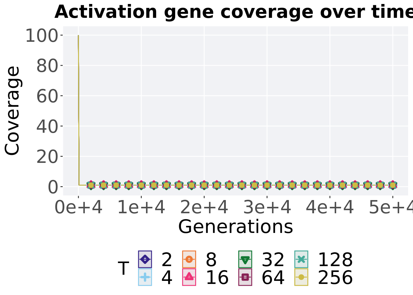

7.3.2.2 End of 50,000 generations

Activation gene coverage in the population at the end of 50,000 generations.

filter(tor_ot, diagnostic == 'contradictory_objectives' & gen == 50000) %>%
ggplot(., aes(x = T, y = uni_str_pos, color = T, fill = T, shape = T)) +
  geom_flat_violin(position = position_nudge(x = .2, y = 0), scale = 'width', alpha = 0.2) +
  geom_point(position = position_jitter(width = .1), size = 1.5, alpha = 1.0) +
  geom_boxplot(color = 'black', width = .2, outlier.shape = NA, alpha = 0.0) +
  scale_y_continuous(
    name="Coverage"
  ) +
  scale_x_discrete(
    name="T"
  )+
  scale_shape_manual(values=SHAPE)+
  scale_colour_manual(values = cb_palette) +
  scale_fill_manual(values = cb_palette) +
  ggtitle("Final activation gene coverage") +
  p_theme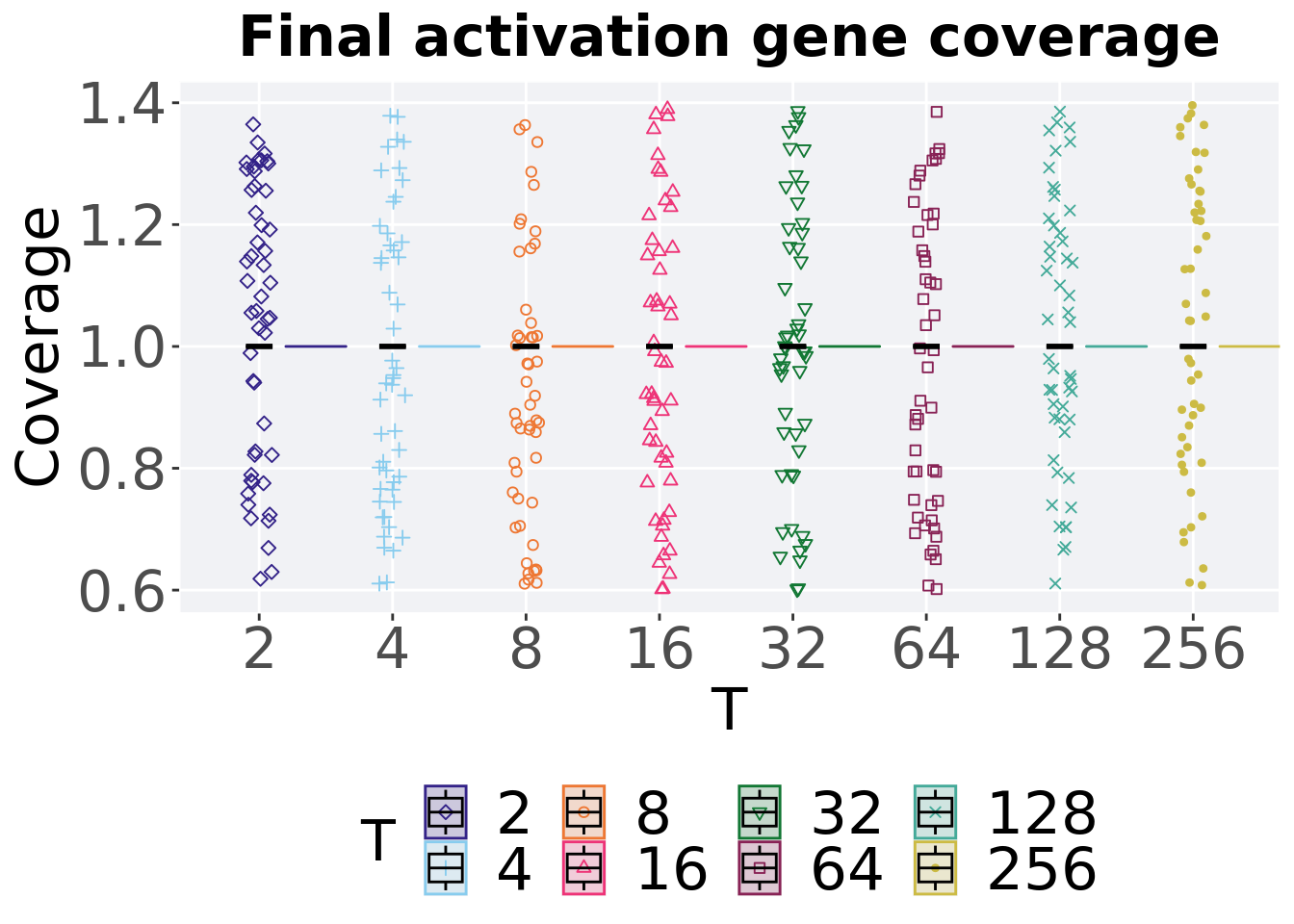

7.3.2.2.1 Stats

Summary statistics for activation gene coverage in the population at the end of 50,000 generations.

coverage = filter(tor_ot, diagnostic == 'contradictory_objectives' & gen == 50000)
group_by(coverage, T) %>%
  dplyr::summarise(
    count = n(),
    na_cnt = sum(is.na(uni_str_pos)),
    min = min(uni_str_pos, na.rm = TRUE),
    median = median(uni_str_pos, na.rm = TRUE),
    mean = mean(uni_str_pos, na.rm = TRUE),
    max = max(uni_str_pos, na.rm = TRUE),
    IQR = IQR(uni_str_pos, na.rm = TRUE)
  )

## # A tibble: 8 x 8
##   T     count na_cnt   min median  mean   max   IQR
##   <fct> <int>  <int> <int>  <dbl> <dbl> <int> <dbl>
## 1 2        50      0     1      1     1     1     0
## 2 4        50      0     1      1     1     1     0
## 3 8        50      0     1      1     1     1     0
## 4 16       50      0     1      1     1     1     0
## 5 32       50      0     1      1     1     1     0
## 6 64       50      0     1      1     1     1     0
## 7 128      50      0     1      1     1     1     0
## 8 256      50      0     1      1     1     1     0

7.3.3 Multi-valley crossing

7.3.3.1 Satisfactory trait coverage over time

lines = filter(tor_ot_mvc, diagnostic == 'contradictory_objectives') %>%
  group_by(T, gen) %>%
  dplyr::summarise(
    min = min(pop_uni_obj),
    mean = mean(pop_uni_obj),
    max = max(pop_uni_obj)
  )

## `summarise()` has grouped output by 'T'. You can override using the `.groups`
## argument.

ggplot(lines, aes(x=gen, y=mean, group = T, fill =T, color = T, shape = T)) +
  geom_ribbon(aes(ymin = min, ymax = max), alpha = 0.1) +
  geom_line(size = 0.5) +
  geom_point(data = filter(lines, gen %% 2000 == 0 & gen != 0), size = 1.5, stroke = 2.0, alpha = 1.0) +
  scale_y_continuous(
    name="Coverage"
  ) +
  scale_x_continuous(
    name="Generations",
    limits=c(0, 50000),
    breaks=c(0, 10000, 20000, 30000, 40000, 50000),
    labels=c("0e+4", "1e+4", "2e+4", "3e+4", "4e+4", "5e+4")

  ) +
  scale_shape_manual(values=SHAPE)+
  scale_colour_manual(values = cb_palette) +
  scale_fill_manual(values = cb_palette) +
  ggtitle("Satisfactory trait coverage over time") +
  p_theme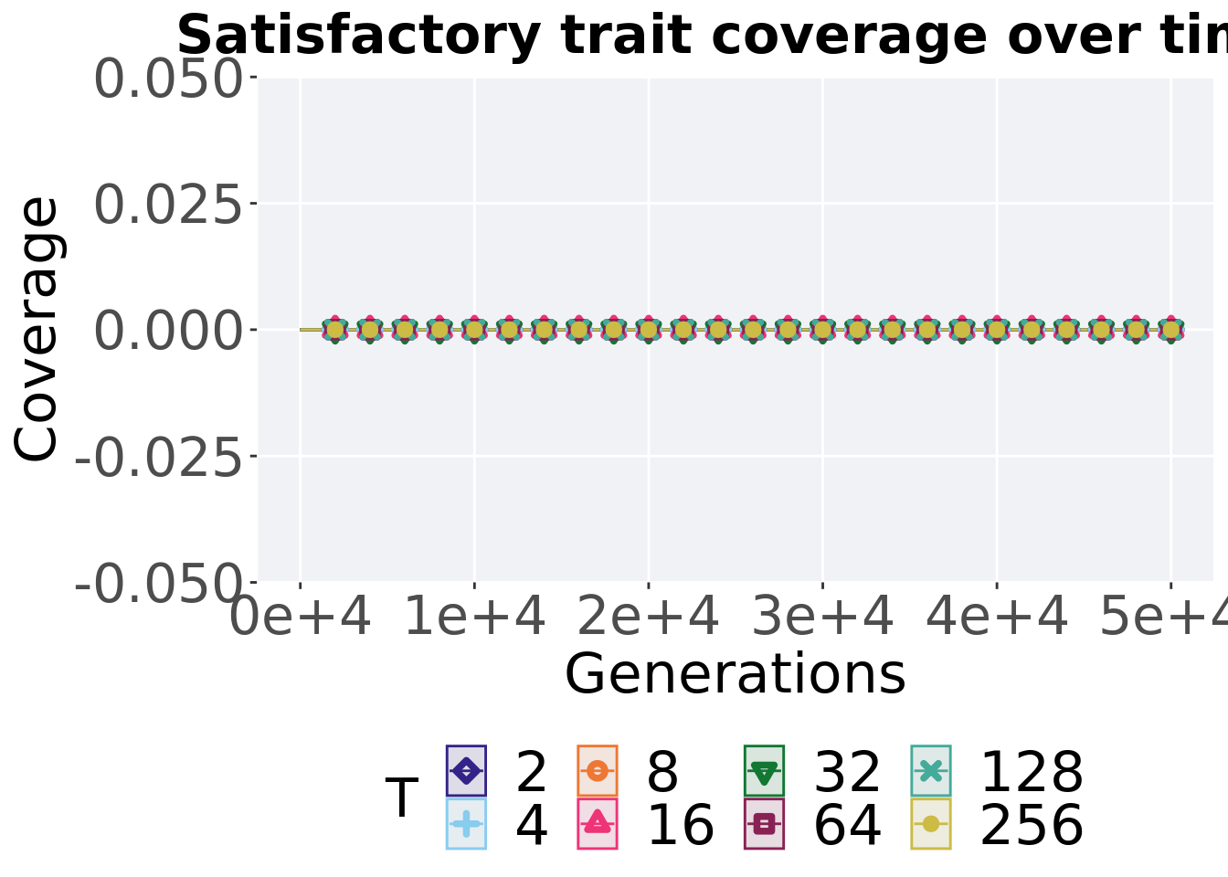

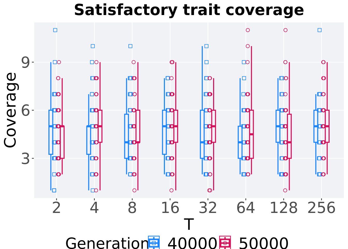
7.3.3.2 Satisfactory trait coverage comparison

Best performances in the population at 40,000 and 50,000 generations.

# 80% and final generation comparison
end = filter(tor_ot_mvc, diagnostic == 'contradictory_objectives' & gen == 50000)
end$Generation <- factor(end$gen)

mid = filter(tor_ot_mvc, diagnostic == 'contradictory_objectives' & gen == 40000)
mid$Generation <- factor(mid$gen)

mvc_p = ggplot(mid, aes(x = T, y=pop_uni_obj, group = T, shape = Generation)) +
  geom_point(col = mvc_col[1] , position = position_jitternudge(jitter.width = .03, nudge.x = -0.05), size = 2, alpha = 1.0) +
  geom_boxplot(position = position_nudge(x = -.15, y = 0), lwd = 0.7, col = mvc_col[1], fill = mvc_col[1], width = .1, outlier.shape = NA, alpha = 0.0) +

  geom_point(data = end, aes(x = T, y=pop_uni_obj), col = mvc_col[2], position = position_jitternudge(jitter.width = .03, nudge.x = 0.05), size = 2, alpha = 1.0) +
  geom_boxplot(data = end, aes(x = T, y=pop_uni_obj), position = position_nudge(x = .15, y = 0), lwd = 0.7, col = mvc_col[2], fill = mvc_col[2], width = .1, outlier.shape = NA, alpha = 0.0) +

  scale_y_continuous(
    name="Coverage",
  ) +
  scale_x_discrete(
    name="T"
  )+
  scale_shape_manual(values=c(0,1))+
  scale_colour_manual(values = c(mvc_col[1],mvc_col[2])) +
  p_theme

plot_grid(
  mvc_p +
    ggtitle("Satisfactory trait coverage") +
    theme(legend.position="none"),
  legend,
  nrow=2,
  rel_heights = c(1,.05),
  label_size = TSIZE
)

7.3.3.2.1 Stats

Summary statistics for the performance of the best performance at 40,000 and 50,000 generations.

slices = filter(tor_ot_mvc, diagnostic == 'contradictory_objectives' & (gen == 50000 | gen == 40000))
slices$Generation <- factor(slices$gen, levels = c(50000,40000))
slices %>%
  group_by(T, Generation) %>%
  dplyr::summarise(
    count = n(),
    na_cnt = sum(is.na(pop_uni_obj)),
    min = min(pop_uni_obj, na.rm = TRUE),
    median = median(pop_uni_obj, na.rm = TRUE),
    mean = mean(pop_uni_obj, na.rm = TRUE),
    max = max(pop_uni_obj, na.rm = TRUE),
    IQR = IQR(pop_uni_obj, na.rm = TRUE)
  )

## `summarise()` has grouped output by 'T'. You can override using the `.groups`
## argument.

## # A tibble: 16 x 9
## # Groups:   T [8]
##    T     Generation count na_cnt   min median  mean   max   IQR
##    <fct> <fct>      <int>  <int> <int>  <dbl> <dbl> <int> <dbl>
##  1 2     50000         50      0     0      0     0     0     0
##  2 2     40000         50      0     0      0     0     0     0
##  3 4     50000         50      0     0      0     0     0     0
##  4 4     40000         50      0     0      0     0     0     0
##  5 8     50000         50      0     0      0     0     0     0
##  6 8     40000         50      0     0      0     0     0     0
##  7 16    50000         50      0     0      0     0     0     0
##  8 16    40000         50      0     0      0     0     0     0
##  9 32    50000         50      0     0      0     0     0     0
## 10 32    40000         50      0     0      0     0     0     0
## 11 64    50000         50      0     0      0     0     0     0
## 12 64    40000         50      0     0      0     0     0     0
## 13 128   50000         50      0     0      0     0     0     0
## 14 128   40000         50      0     0      0     0     0     0
## 15 256   50000         50      0     0      0     0     0     0
## 16 256   40000         50      0     0      0     0     0     0

T 2

wilcox.test(x = filter(slices, T == 2 & Generation == 50000)$pop_uni_obj,
            y = filter(slices, T == 2 & Generation == 40000)$pop_uni_obj,
            alternative = 't')

## 
##  Wilcoxon rank sum test with continuity correction
## 
## data:  filter(slices, T == 2 & Generation == 50000)$pop_uni_obj and filter(slices, T == 2 & Generation == 40000)$pop_uni_obj
## W = 1250, p-value = NA
## alternative hypothesis: true location shift is not equal to 0

T 4

wilcox.test(x = filter(slices, T == 4 & Generation == 50000)$pop_uni_obj,
            y = filter(slices, T == 4 & Generation == 40000)$pop_uni_obj,
            alternative = 't')

## 
##  Wilcoxon rank sum test with continuity correction
## 
## data:  filter(slices, T == 4 & Generation == 50000)$pop_uni_obj and filter(slices, T == 4 & Generation == 40000)$pop_uni_obj
## W = 1250, p-value = NA
## alternative hypothesis: true location shift is not equal to 0

T 8

wilcox.test(x = filter(slices, T == 8 & Generation == 50000)$pop_uni_obj,
            y = filter(slices, T == 8 & Generation == 40000)$pop_uni_obj,
            alternative = 't')

## 
##  Wilcoxon rank sum test with continuity correction
## 
## data:  filter(slices, T == 8 & Generation == 50000)$pop_uni_obj and filter(slices, T == 8 & Generation == 40000)$pop_uni_obj
## W = 1250, p-value = NA
## alternative hypothesis: true location shift is not equal to 0

T 16

wilcox.test(x = filter(slices, T == 16 & Generation == 50000)$pop_uni_obj,
            y = filter(slices, T == 16 & Generation == 40000)$pop_uni_obj,
            alternative = 't')

## 
##  Wilcoxon rank sum test with continuity correction
## 
## data:  filter(slices, T == 16 & Generation == 50000)$pop_uni_obj and filter(slices, T == 16 & Generation == 40000)$pop_uni_obj
## W = 1250, p-value = NA
## alternative hypothesis: true location shift is not equal to 0

T 32

wilcox.test(x = filter(slices, T == 32 & Generation == 50000)$pop_uni_obj,
            y = filter(slices, T == 32 & Generation == 40000)$pop_uni_obj,
            alternative = 't')

## 
##  Wilcoxon rank sum test with continuity correction
## 
## data:  filter(slices, T == 32 & Generation == 50000)$pop_uni_obj and filter(slices, T == 32 & Generation == 40000)$pop_uni_obj
## W = 1250, p-value = NA
## alternative hypothesis: true location shift is not equal to 0

T 64

wilcox.test(x = filter(slices, T == 64 & Generation == 50000)$pop_uni_obj,
            y = filter(slices, T == 64 & Generation == 40000)$pop_uni_obj,
            alternative = 't')

## 
##  Wilcoxon rank sum test with continuity correction
## 
## data:  filter(slices, T == 64 & Generation == 50000)$pop_uni_obj and filter(slices, T == 64 & Generation == 40000)$pop_uni_obj
## W = 1250, p-value = NA
## alternative hypothesis: true location shift is not equal to 0

T 128

wilcox.test(x = filter(slices, T == 128 & Generation == 50000)$pop_uni_obj,
            y = filter(slices, T == 128 & Generation == 40000)$pop_uni_obj,
            alternative = 't')

## 
##  Wilcoxon rank sum test with continuity correction
## 
## data:  filter(slices, T == 128 & Generation == 50000)$pop_uni_obj and filter(slices, T == 128 & Generation == 40000)$pop_uni_obj
## W = 1250, p-value = NA
## alternative hypothesis: true location shift is not equal to 0

T 256

wilcox.test(x = filter(slices, T == 256 & Generation == 50000)$pop_uni_obj,
            y = filter(slices, T == 256 & Generation == 40000)$pop_uni_obj,
            alternative = 't')

## 
##  Wilcoxon rank sum test with continuity correction
## 
## data:  filter(slices, T == 256 & Generation == 50000)$pop_uni_obj and filter(slices, T == 256 & Generation == 40000)$pop_uni_obj
## W = 1250, p-value = NA
## alternative hypothesis: true location shift is not equal to 0

7.3.3.3 Activation gene coverage over time

lines = filter(tor_ot_mvc, diagnostic == 'contradictory_objectives') %>%
  group_by(T, gen) %>%
  dplyr::summarise(
    min = min(uni_str_pos),
    mean = mean(uni_str_pos),
    max = max(uni_str_pos)
  )

## `summarise()` has grouped output by 'T'. You can override using the `.groups`
## argument.

ggplot(lines, aes(x=gen, y=mean, group = T, fill =T, color = T, shape = T)) +
  geom_ribbon(aes(ymin = min, ymax = max), alpha = 0.1) +
  geom_line(size = 0.5) +
  geom_point(data = filter(lines, gen %% 2000 == 0 & gen != 0), size = 1.5, stroke = 2.0, alpha = 1.0) +
  scale_y_continuous(
    name="Coverage"
  ) +
  scale_x_continuous(
    name="Generations",
    limits=c(0, 50000),
    breaks=c(0, 10000, 20000, 30000, 40000, 50000),
    labels=c("0e+4", "1e+4", "2e+4", "3e+4", "4e+4", "5e+4")

  ) +
  scale_shape_manual(values=SHAPE)+
  scale_colour_manual(values = cb_palette) +
  scale_fill_manual(values = cb_palette) +
  ggtitle("Activation gene coverage over time") +
  p_theme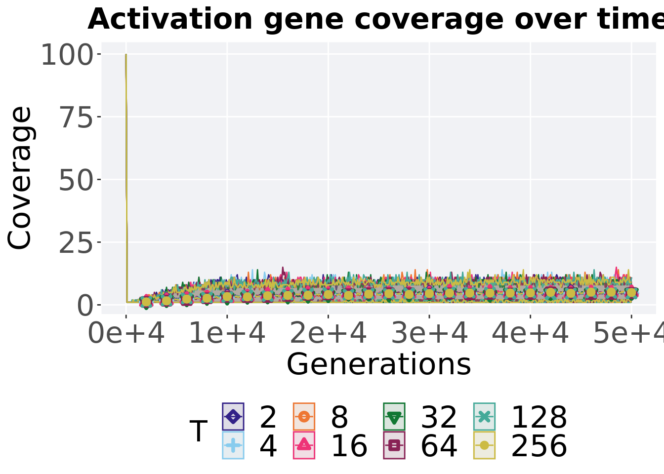

7.3.3.4 Activation gene coverage comparison

Activation gene coverage in the population at 40,000 and 50,000 generations.

# 80% and final generation comparison
end = filter(tor_ot_mvc, diagnostic == 'contradictory_objectives' & gen == 50000)
end$Generation <- factor(end$gen)

mid = filter(tor_ot_mvc, diagnostic == 'contradictory_objectives' & gen == 40000)
mid$Generation <- factor(mid$gen)

mvc_p = ggplot(mid, aes(x = T, y=uni_str_pos, group = T, shape = Generation)) +
  geom_point(col = mvc_col[1] , position = position_jitternudge(jitter.width = .03, nudge.x = -0.05), size = 2, alpha = 1.0) +
  geom_boxplot(position = position_nudge(x = -.15, y = 0), lwd = 0.7, col = mvc_col[1], fill = mvc_col[1], width = .1, outlier.shape = NA, alpha = 0.0) +

  geom_point(data = end, aes(x = T, y=uni_str_pos), col = mvc_col[2], position = position_jitternudge(jitter.width = .03, nudge.x = 0.05), size = 2, alpha = 1.0) +
  geom_boxplot(data = end, aes(x = T, y=uni_str_pos), position = position_nudge(x = .15, y = 0), lwd = 0.7, col = mvc_col[2], fill = mvc_col[2], width = .1, outlier.shape = NA, alpha = 0.0) +

  scale_y_continuous(
    name="Coverage",
  ) +
  scale_x_discrete(
    name="T"
  )+
  scale_shape_manual(values=c(0,1))+
  scale_colour_manual(values = c(mvc_col[1],mvc_col[2])) +
  p_theme

plot_grid(
  mvc_p +
    ggtitle("Satisfactory trait coverage") +
    theme(legend.position="none"),
  legend,
  nrow=2,
  rel_heights = c(1,.05),
  label_size = TSIZE
)

7.3.3.4.1 Stats

Summary statistics for the activation gene coverage at 40,000 and 50,000 generations.

slices = filter(tor_ot_mvc, diagnostic == 'contradictory_objectives' & (gen == 50000 | gen == 40000))
slices$Generation <- factor(slices$gen, levels = c(50000,40000))
slices %>%
  group_by(T, Generation) %>%
  dplyr::summarise(
    count = n(),
    na_cnt = sum(is.na(uni_str_pos)),
    min = min(uni_str_pos, na.rm = TRUE),
    median = median(uni_str_pos, na.rm = TRUE),
    mean = mean(uni_str_pos, na.rm = TRUE),
    max = max(uni_str_pos, na.rm = TRUE),
    IQR = IQR(uni_str_pos, na.rm = TRUE)
  )

## `summarise()` has grouped output by 'T'. You can override using the `.groups`
## argument.

## # A tibble: 16 x 9
## # Groups:   T [8]
##    T     Generation count na_cnt   min median  mean   max   IQR
##    <fct> <fct>      <int>  <int> <int>  <dbl> <dbl> <int> <dbl>
##  1 2     50000         50      0     2    5    4.6      9  2   
##  2 2     40000         50      0     1    5    4.7     11  2.75
##  3 4     50000         50      0     1    5    4.86     9  2   
##  4 4     40000         50      0     1    5    4.68    10  1.75
##  5 8     50000         50      0     1    4    4.64     9  2   
##  6 8     40000         50      0     2    4    4.54    10  2.75
##  7 16    50000         50      0     1    5    4.92     9  2   
##  8 16    40000         50      0     2    5    4.74     8  2.75
##  9 32    50000         50      0     1    5    4.86     8  2   
## 10 32    40000         50      0     2    4    4.6     10  3   
## 11 64    50000         50      0     2    4.5  4.74    11  3   
## 12 64    40000         50      0     2    4    4.34     9  2   
## 13 128   50000         50      0     1    4    4.52    11  2.75
## 14 128   40000         50      0     2    5    4.78     8  2   
## 15 256   50000         50      0     2    5    4.92     9  2   
## 16 256   40000         50      0     2    5    4.78    11  2

T 2

wilcox.test(x = filter(slices, T == 2 & Generation == 50000)$uni_str_pos,
            y = filter(slices, T == 2 & Generation == 40000)$uni_str_pos,
            alternative = 't')

## 
##  Wilcoxon rank sum test with continuity correction
## 
## data:  filter(slices, T == 2 & Generation == 50000)$uni_str_pos and filter(slices, T == 2 & Generation == 40000)$uni_str_pos
## W = 1205, p-value = 0.7547
## alternative hypothesis: true location shift is not equal to 0

T 4

wilcox.test(x = filter(slices, T == 4 & Generation == 50000)$uni_str_pos,
            y = filter(slices, T == 4 & Generation == 40000)$uni_str_pos,
            alternative = 't')

## 
##  Wilcoxon rank sum test with continuity correction
## 
## data:  filter(slices, T == 4 & Generation == 50000)$uni_str_pos and filter(slices, T == 4 & Generation == 40000)$uni_str_pos
## W = 1355, p-value = 0.4625
## alternative hypothesis: true location shift is not equal to 0

T 8

wilcox.test(x = filter(slices, T == 8 & Generation == 50000)$uni_str_pos,
            y = filter(slices, T == 8 & Generation == 40000)$uni_str_pos,
            alternative = 't')

## 
##  Wilcoxon rank sum test with continuity correction
## 
## data:  filter(slices, T == 8 & Generation == 50000)$uni_str_pos and filter(slices, T == 8 & Generation == 40000)$uni_str_pos
## W = 1351.5, p-value = 0.4781
## alternative hypothesis: true location shift is not equal to 0

T 16

wilcox.test(x = filter(slices, T == 16 & Generation == 50000)$uni_str_pos,
            y = filter(slices, T == 16 & Generation == 40000)$uni_str_pos,
            alternative = 't')

## 
##  Wilcoxon rank sum test with continuity correction
## 
## data:  filter(slices, T == 16 & Generation == 50000)$uni_str_pos and filter(slices, T == 16 & Generation == 40000)$uni_str_pos
## W = 1310, p-value = 0.677
## alternative hypothesis: true location shift is not equal to 0

T 32

wilcox.test(x = filter(slices, T == 32 & Generation == 50000)$uni_str_pos,
            y = filter(slices, T == 32 & Generation == 40000)$uni_str_pos,
            alternative = 't')

## 
##  Wilcoxon rank sum test with continuity correction
## 
## data:  filter(slices, T == 32 & Generation == 50000)$uni_str_pos and filter(slices, T == 32 & Generation == 40000)$uni_str_pos
## W = 1383, p-value = 0.3552
## alternative hypothesis: true location shift is not equal to 0

T 64

wilcox.test(x = filter(slices, T == 64 & Generation == 50000)$uni_str_pos,
            y = filter(slices, T == 64 & Generation == 40000)$uni_str_pos,
            alternative = 't')

## 
##  Wilcoxon rank sum test with continuity correction
## 
## data:  filter(slices, T == 64 & Generation == 50000)$uni_str_pos and filter(slices, T == 64 & Generation == 40000)$uni_str_pos
## W = 1373.5, p-value = 0.3871
## alternative hypothesis: true location shift is not equal to 0

T 128

wilcox.test(x = filter(slices, T == 128 & Generation == 50000)$uni_str_pos,
            y = filter(slices, T == 128 & Generation == 40000)$uni_str_pos,
            alternative = 't')

## 
##  Wilcoxon rank sum test with continuity correction
## 
## data:  filter(slices, T == 128 & Generation == 50000)$uni_str_pos and filter(slices, T == 128 & Generation == 40000)$uni_str_pos
## W = 1078, p-value = 0.2303
## alternative hypothesis: true location shift is not equal to 0

T 256

wilcox.test(x = filter(slices, T == 256 & Generation == 50000)$uni_str_pos,
            y = filter(slices, T == 256 & Generation == 40000)$uni_str_pos,
            alternative = 't')

## 
##  Wilcoxon rank sum test with continuity correction
## 
## data:  filter(slices, T == 256 & Generation == 50000)$uni_str_pos and filter(slices, T == 256 & Generation == 40000)$uni_str_pos
## W = 1280, p-value = 0.8358
## alternative hypothesis: true location shift is not equal to 0

7.4 Multi-path exploration results

Here we present the results for best performances and activation gene coverage found by each tournament selection size value replicate on the multi-path exploration diagnostic. Best performance found refers to the largest average trait score found in a given population, while activation gene coverage refers to the count of unique activation genes in the population. Note that both values fall between 0 and 100.

7.4.1 Performance

Here we analyze the performances for each parameter replicate on the multi-path exploration diagnostic.

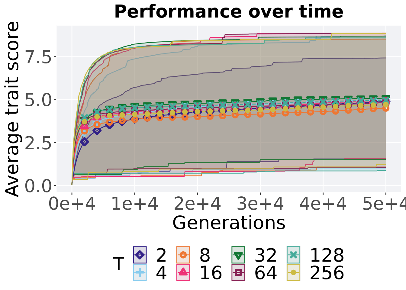
7.4.1.1 Performance over time

Performance over time.

lines = filter(tor_ot, diagnostic == 'multipath_exploration') %>%
        group_by(T, gen) %>%
          dplyr::summarise(
            min = min(pop_fit_max),
            mean = mean(pop_fit_max),
            max = max(pop_fit_max)
          )

## `summarise()` has grouped output by 'T'. You can override using the `.groups`
## argument.

ggplot(lines, aes(x=gen, y=mean / DIMENSIONALITY, group = T, fill = T, color = T, shape = T)) +
  geom_ribbon(aes(ymin = min / DIMENSIONALITY, ymax = max / DIMENSIONALITY), alpha = 0.1) +
  geom_line(size = 0.5) +
  geom_point(data = filter(lines, gen %% 2000 == 0 & gen != 0), size = 1.5, stroke = 2.0, alpha = 1.0) +
  scale_y_continuous(
    name="Average trait score",
    limits=c(-1, 101),
    breaks=seq(0,100, 20),
    labels=c("0", "20", "40", "60", "80", "100")
  ) +
  scale_x_continuous(
    name="Generations",
    limits=c(0, 50000),
    breaks=c(0, 10000, 20000, 30000, 40000, 50000),
    labels=c("0e+4", "1e+4", "2e+4", "3e+4", "4e+4", "5e+4")

  ) +
  scale_shape_manual(values=SHAPE)+
  scale_colour_manual(values = cb_palette) +
  scale_fill_manual(values = cb_palette) +
  ggtitle("Best performance over time") +
  p_theme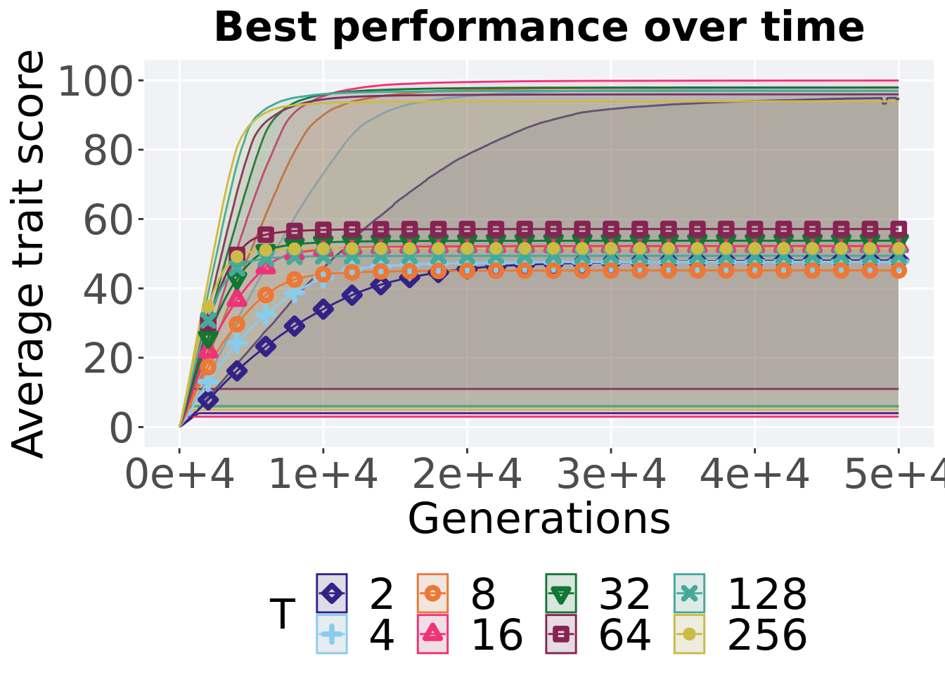

7.4.1.2 Best performance throughout

Here we plot the performance of the best performing solution found throughout 50,000 generations.

performance = filter(tor_best, col == 'pop_fit_max' & diagnostic == 'multipath_exploration') %>%
ggplot(., aes(x = T, y = val / DIMENSIONALITY, color = T, fill = T, shape = T)) +
  geom_flat_violin(position = position_nudge(x = .2, y = 0), scale = 'width', alpha = 0.2) +
  geom_point(position = position_jitter(width = .1), size = 1.5, alpha = 1.0) +
  geom_boxplot(color = 'black', width = .2, outlier.shape = NA, alpha = 0.0) +
  scale_y_continuous(
    name="Average trait score",
    limits=c(-1, 101),
    breaks=seq(0,100, 20),
    labels=c("0", "20", "40", "60", "80", "100")
  ) +
  scale_x_discrete(
    name="T"
  )+
  scale_shape_manual(values=SHAPE)+
  scale_colour_manual(values = cb_palette) +
  scale_fill_manual(values = cb_palette) +
  p_theme

7.4.1.2.1 Stats

Summary statistics for the performance of the best performing solution found throughout 50,000 generations.

performance = filter(tor_best, col == 'pop_fit_max' & diagnostic == 'multipath_exploration')
group_by(performance, T) %>%
  dplyr::summarise(
    count = n(),
    na_cnt = sum(is.na(val)),
    min = min(val / DIMENSIONALITY, na.rm = TRUE),
    median = median(val / DIMENSIONALITY, na.rm = TRUE),
    mean = mean(val / DIMENSIONALITY, na.rm = TRUE),
    max = max(val / DIMENSIONALITY, na.rm = TRUE),
    IQR = IQR(val / DIMENSIONALITY, na.rm = TRUE)
  )

## # A tibble: 8 x 8
##   T     count na_cnt   min median  mean   max   IQR
##   <fct> <int>  <int> <dbl>  <dbl> <dbl> <dbl> <dbl>
## 1 2        50      0  4      52.5  48.1  95.0  43.4
## 2 4        50      0  5      45.0  47.7  97.8  58.2
## 3 8        50      0  6.00   42.5  45.2  97.9  53.2
## 4 16       50      0  3      48.0  52.2 100.   61.5
## 5 32       50      0  6      53.0  53.8  98.0  55.2
## 6 64       50      0 11      58.0  57.1  96.0  44.0
## 7 128      50      0  6.00   52.0  49.4  97.0  47.0
## 8 256      50      0  5      51.0  51.5  94.0  41.5

Kruskal–Wallis test provides evidence of no statistical differences among the best performing solution found throughout 50,000 generations.

kruskal.test(val ~ T,data = performance)

## 
##  Kruskal-Wallis rank sum test
## 
## data:  val by T
## Kruskal-Wallis chi-squared = 6.9356, df = 7, p-value = 0.4356

7.4.1.3 End of 50,000 generations

Best performance in the population at the end of 50,000 generations.

filter(tor_ot, diagnostic == 'multipath_exploration' & gen == 50000) %>%
ggplot(., aes(x = T, y = pop_fit_max / DIMENSIONALITY, color = T, fill = T, shape = T)) +
  geom_flat_violin(position = position_nudge(x = .2, y = 0), scale = 'width', alpha = 0.2) +
  geom_point(position = position_jitter(width = .1), size = 1.5, alpha = 1.0) +
  geom_boxplot(color = 'black', width = .2, outlier.shape = NA, alpha = 0.0) +
  scale_y_continuous(
    name="Average trait score",
    limits=c(-1, 101),
    breaks=seq(0,100, 20),
    labels=c("0", "20", "40", "60", "80", "100")
  ) +
  scale_x_discrete(
    name="T"
  )+
  scale_shape_manual(values=SHAPE)+
  scale_colour_manual(values = cb_palette) +
  scale_fill_manual(values = cb_palette) +
  ggtitle("Final performance") +
  p_theme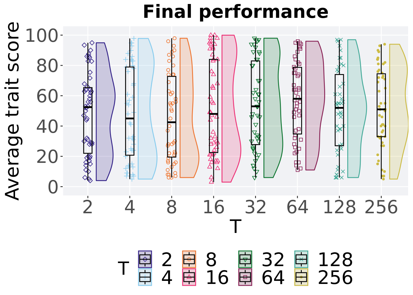

7.4.1.3.1 Stats

Summary statistics for the best performance in the population at the end of 50,000 generations.

performance = filter(tor_ot, diagnostic == 'multipath_exploration' & gen == 50000)
group_by(performance, T) %>%
  dplyr::summarise(
    count = n(),
    na_cnt = sum(is.na(pop_fit_max / DIMENSIONALITY)),
    min = min(pop_fit_max / DIMENSIONALITY, na.rm = TRUE),
    median = median(pop_fit_max / DIMENSIONALITY, na.rm = TRUE),
    mean = mean(pop_fit_max / DIMENSIONALITY, na.rm = TRUE),
    max = max(pop_fit_max / DIMENSIONALITY, na.rm = TRUE),
    IQR = IQR(pop_fit_max / DIMENSIONALITY, na.rm = TRUE)
  )

## # A tibble: 8 x 8
##   T     count na_cnt   min median  mean   max   IQR
##   <fct> <int>  <int> <dbl>  <dbl> <dbl> <dbl> <dbl>
## 1 2        50      0  4      52.5  48.1  94.9  43.4
## 2 4        50      0  5      45.0  47.7  97.8  58.2
## 3 8        50      0  6.00   42.5  45.2  97.9  53.2
## 4 16       50      0  3      48.0  52.2 100.   61.5
## 5 32       50      0  6      53.0  53.8  98.0  55.2
## 6 64       50      0 11      58.0  57.1  96.0  44.0
## 7 128      50      0  6.00   52.0  49.4  97.0  47.0
## 8 256      50      0  5      51.0  51.5  94.0  41.5

Kruskal–Wallis test provides evidence of statistical differences among best performance in the population at the end of 50,000 generations.

kruskal.test(pop_fit_max ~ T, data = performance)

## 
##  Kruskal-Wallis rank sum test
## 
## data:  pop_fit_max by T
## Kruskal-Wallis chi-squared = 6.9356, df = 7, p-value = 0.4356

Results for post-hoc Wilcoxon rank-sum test with a Bonferroni correction on the best performance in the population at the end of 50,000 generations.

pairwise.wilcox.test(x = performance$pop_fit_max, g = performance$T , p.adjust.method = "bonferroni",
                     paired = FALSE, conf.int = FALSE, alternative = 'l')

## 
##  Pairwise comparisons using Wilcoxon rank sum test with continuity correction 
## 
## data:  performance$pop_fit_max and performance$T 
## 
##     2 4 8 16 32 64 128
## 4   1 - - -  -  -  -  
## 8   1 1 - -  -  -  -  
## 16  1 1 1 -  -  -  -  
## 32  1 1 1 1  -  -  -  
## 64  1 1 1 1  1  -  -  
## 128 1 1 1 1  1  1  -  
## 256 1 1 1 1  1  1  1  
## 
## P value adjustment method: bonferroni

7.4.2 Activation gene coverage

Here we analyze the activation gene coverage for each parameter replicate on the multi-path exploration diagnostic.

7.4.2.1 Coverage over time

Activation gene coverage over time.

lines = filter(tor_ot, diagnostic == 'multipath_exploration') %>%
        group_by(T, gen) %>%
          dplyr::summarise(
            min = min(uni_str_pos),
            mean = mean(uni_str_pos),
            max = max(uni_str_pos)
          )

## `summarise()` has grouped output by 'T'. You can override using the `.groups`
## argument.

ggplot(lines, aes(x=gen, y=mean, group = T, fill =T, color = T, shape = T)) +
  geom_ribbon(aes(ymin = min, ymax = max), alpha = 0.1) +
  geom_line(size = 0.5) +
  geom_point(data = filter(lines, gen %% 2000 == 0 & gen != 0), size = 1.5, stroke = 2.0, alpha = 1.0) +
  scale_y_continuous(
    name="Coverage",
    limits=c(-1, 101),
    breaks=seq(0,100, 20),
    labels=c("0", "20", "40", "60", "80", "100")
  ) +
  scale_x_continuous(
    name="Generations",
    limits=c(0, 50000),
    breaks=c(0, 10000, 20000, 30000, 40000, 50000),
    labels=c("0e+4", "1e+4", "2e+4", "3e+4", "4e+4", "5e+4")

  ) +
  scale_shape_manual(values=SHAPE)+
  scale_colour_manual(values = cb_palette) +
  scale_fill_manual(values = cb_palette) +
  ggtitle("Activation gene coverage over time") +
  p_theme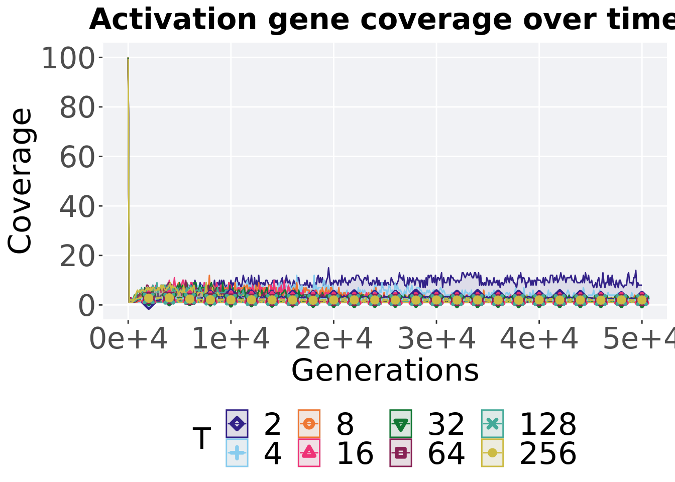

7.4.2.2 End of 50,000 generations

Activation gene coverage in the population at the end of 50,000 generations.

filter(tor_ot, diagnostic == 'multipath_exploration' & gen == 50000) %>%
ggplot(., aes(x = T, y = uni_str_pos, color = T, fill = T, shape = T)) +
  geom_flat_violin(position = position_nudge(x = .2, y = 0), scale = 'width', alpha = 0.2) +
  geom_point(position = position_jitter(width = .1), size = 1.5, alpha = 1.0) +
  geom_boxplot(color = 'black', width = .2, outlier.shape = NA, alpha = 0.0) +
  scale_y_continuous(
    name="Coverage"
  ) +
  scale_x_discrete(
    name="T"
  )+
  scale_shape_manual(values=SHAPE)+
  scale_colour_manual(values = cb_palette) +
  scale_fill_manual(values = cb_palette) +
  ggtitle("Final activation gene coverage") +
  p_theme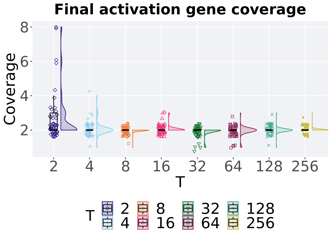

7.4.2.2.1 Stats

Summary statistics for the activation gene coverage in the population at the end of 50,000 generations.

coverage = filter(tor_ot, diagnostic == 'multipath_exploration' & gen == 50000)
group_by(coverage, T) %>%
  dplyr::summarise(
    count = n(),
    na_cnt = sum(is.na(uni_str_pos)),
    min = min(uni_str_pos, na.rm = TRUE),
    median = median(uni_str_pos, na.rm = TRUE),
    mean = mean(uni_str_pos, na.rm = TRUE),
    max = max(uni_str_pos, na.rm = TRUE),
    IQR = IQR(uni_str_pos, na.rm = TRUE)
  )

## # A tibble: 8 x 8
##   T     count na_cnt   min median  mean   max   IQR
##   <fct> <int>  <int> <int>  <dbl> <dbl> <int> <dbl>
## 1 2        50      0     2      2  2.68     8     1
## 2 4        50      0     1      2  2.08     4     0
## 3 8        50      0     1      2  1.98     2     0
## 4 16       50      0     2      2  2.06     3     0
## 5 32       50      0     1      2  1.92     2     0
## 6 64       50      0     1      2  1.94     3     0
## 7 128      50      0     1      2  2        3     0
## 8 256      50      0     2      2  2.02     3     0

Kruskal–Wallis test provides evidence of statistical differences among activation gene coverage in the population at the end of 50,000 generations.

kruskal.test(uni_str_pos ~ T, data = coverage)

## 
##  Kruskal-Wallis rank sum test
## 
## data:  uni_str_pos by T
## Kruskal-Wallis chi-squared = 61.183, df = 7, p-value = 8.757e-11

Results for post-hoc Wilcoxon rank-sum test with a Bonferroni correction on the activation gene coverage in the population at the end of 50,000 generations.

pairwise.wilcox.test(x = coverage$uni_str_pos, g = coverage$T , p.adjust.method = "bonferroni",
                     paired = FALSE, conf.int = FALSE, alternative = 't')

## 
##  Pairwise comparisons using Wilcoxon rank sum test with continuity correction 
## 
## data:  coverage$uni_str_pos and coverage$T 
## 
##     2       4       8       16      32      64      128    
## 4   0.04907 -       -       -       -       -       -      
## 8   0.00031 1.00000 -       -       -       -       -      
## 16  0.02131 1.00000 1.00000 -       -       -       -      
## 32  0.00011 0.58051 1.00000 0.24142 -       -       -      
## 64  0.00044 1.00000 1.00000 0.99216 1.00000 -       -      
## 128 0.00134 1.00000 1.00000 1.00000 1.00000 1.00000 -      
## 256 0.00191 1.00000 1.00000 1.00000 0.70887 1.00000 1.00000
## 
## P value adjustment method: bonferroni

7.4.3 Multi-valley crossing

7.4.3.1 Performance over time

# data for lines and shading on plots
lines = filter(tor_ot_mvc, diagnostic == 'multipath_exploration') %>%
  group_by(T, gen) %>%
  dplyr::summarise(
    min = min(pop_fit_max) / DIMENSIONALITY,
    mean = mean(pop_fit_max) / DIMENSIONALITY,
    max = max(pop_fit_max) / DIMENSIONALITY
  )

## `summarise()` has grouped output by 'T'. You can override using the `.groups`
## argument.

ggplot(lines, aes(x=gen, y=mean, group = T, fill =T, color = T, shape = T)) +
  geom_ribbon(aes(ymin = min, ymax = max), alpha = 0.1) +
  geom_line(size = 0.5) +
  geom_point(data = filter(lines, gen %% 2000 == 0 & gen != 0), size = 1.5, stroke = 2.0, alpha = 1.0) +
  scale_y_continuous(
    name="Average trait score"
  ) +
  scale_x_continuous(
    name="Generations",
    limits=c(0, 50000),
    breaks=c(0, 10000, 20000, 30000, 40000, 50000),
    labels=c("0e+4", "1e+4", "2e+4", "3e+4", "4e+4", "5e+4")

  ) +
  scale_shape_manual(values=SHAPE)+
  scale_colour_manual(values = cb_palette) +
  scale_fill_manual(values = cb_palette) +
  ggtitle('Performance over time')+
  p_theme +
  guides(
    shape=guide_legend(nrow=2, title.position = "left"),
    color=guide_legend(nrow=2, title.position = "left"),
    fill=guide_legend(nrow=2, title.position = "left")
  )

7.4.3.2 Performance comparison

Best performances in the population at 40,000 and 50,000 generations.

# 80% and final generation comparison
end = filter(tor_ot_mvc, diagnostic == 'multipath_exploration' & gen == 50000 & T != 'ran')
end$Generation <- factor(end$gen)

mid = filter(tor_ot_mvc, diagnostic == 'multipath_exploration' & gen == 40000 & T != 'ran')
mid$Generation <- factor(mid$gen)

mvc_p = ggplot(mid, aes(x = T, y=pop_fit_max / DIMENSIONALITY, group = T, shape = Generation)) +
  geom_point(col = mvc_col[1] , position = position_jitternudge(jitter.width = .03, nudge.x = -0.05), size = 2, alpha = 1.0) +
  geom_boxplot(position = position_nudge(x = -.15, y = 0), lwd = 0.7, col = mvc_col[1], fill = mvc_col[1], width = .1, outlier.shape = NA, alpha = 0.0) +

  geom_point(data = end, aes(x = T, y=pop_fit_max / DIMENSIONALITY), col = mvc_col[2], position = position_jitternudge(jitter.width = .03, nudge.x = 0.05), size = 2, alpha = 1.0) +
  geom_boxplot(data = end, aes(x = T, y=pop_fit_max / DIMENSIONALITY), position = position_nudge(x = .15, y = 0), lwd = 0.7, col = mvc_col[2], fill = mvc_col[2], width = .1, outlier.shape = NA, alpha = 0.0) +

  scale_y_continuous(
    name="Average trait score"
  ) +
  scale_x_discrete(
    name="T"
  )+
  scale_shape_manual(values=c(0,1))+
  scale_colour_manual(values = c(mvc_col[1],mvc_col[2])) +
  p_theme

plot_grid(
  mvc_p +
    ggtitle("Performance comparisons") +
    theme(legend.position="none"),
  legend,
  nrow=2,
  rel_heights = c(1,.05),
  label_size = TSIZE
)

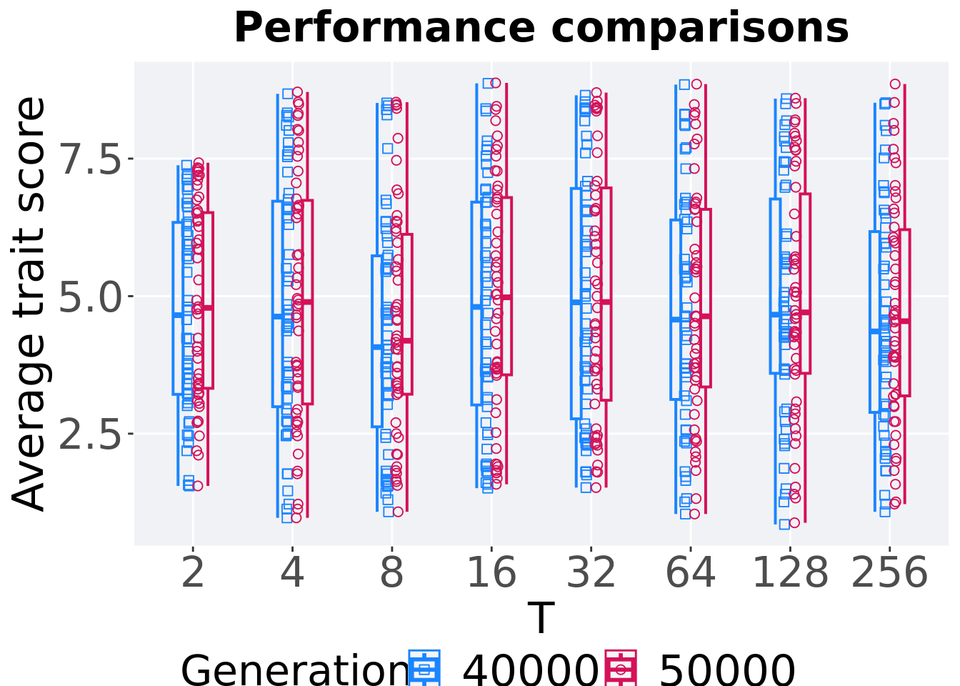
7.4.3.3 Stats

Summary statistics for the performance of the best performance at 40,000 and 50,000 generations.

slices = filter(tor_ot_mvc, diagnostic == 'multipath_exploration' & (gen == 50000 | gen == 40000))
slices$Generation <- factor(slices$gen, levels = c(50000,40000))
slices %>%
  group_by(T, Generation) %>%
  dplyr::summarise(
    count = n(),
    na_cnt = sum(is.na(pop_fit_max  / DIMENSIONALITY)),
    min = min(pop_fit_max  / DIMENSIONALITY, na.rm = TRUE),
    median = median(pop_fit_max  / DIMENSIONALITY, na.rm = TRUE),
    mean = mean(pop_fit_max  / DIMENSIONALITY, na.rm = TRUE),
    max = max(pop_fit_max  / DIMENSIONALITY, na.rm = TRUE),
    IQR = IQR(pop_fit_max  / DIMENSIONALITY, na.rm = TRUE)
  )

## `summarise()` has grouped output by 'T'. You can override using the `.groups`
## argument.

## # A tibble: 16 x 9
## # Groups:   T [8]
##    T     Generation count na_cnt   min median  mean   max   IQR
##    <fct> <fct>      <int>  <int> <dbl>  <dbl> <dbl> <dbl> <dbl>
##  1 2     50000         50      0 1.55    4.79  4.89  7.43  3.19
##  2 2     40000         50      0 1.55    4.65  4.68  7.38  3.13
##  3 4     50000         50      0 0.970   4.89  4.98  8.71  3.70
##  4 4     40000         50      0 0.970   4.63  4.87  8.68  3.74
##  5 8     50000         50      0 1.08    4.19  4.50  8.53  2.91
##  6 8     40000         50      0 1.08    4.07  4.31  8.51  3.11
##  7 16    50000         50      0 1.58    4.98  4.94  8.88  3.22
##  8 16    40000         50      0 1.51    4.80  4.80  8.87  3.69
##  9 32    50000         50      0 1.52    4.89  5.09  8.70  3.86
## 10 32    40000         50      0 1.52    4.89  5.02  8.65  4.19
## 11 64    50000         50      0 1.04    4.63  4.84  8.85  3.23
## 12 64    40000         50      0 1.04    4.57  4.71  8.85  3.26
## 13 128   50000         50      0 0.880   4.70  4.96  8.60  3.26
## 14 128   40000         50      0 0.850   4.66  4.88  8.59  3.17
## 15 256   50000         50      0 1.22    4.54  4.70  8.86  3.02
## 16 256   40000         50      0 1.08    4.36  4.57  8.51  3.29

T 2

wilcox.test(x = filter(slices, T == 2 & Generation == 50000)$pop_fit_max,
            y = filter(slices, T == 2 & Generation == 40000)$pop_fit_max,
            alternative = 't')

## 
##  Wilcoxon rank sum test with continuity correction
## 
## data:  filter(slices, T == 2 & Generation == 50000)$pop_fit_max and filter(slices, T == 2 & Generation == 40000)$pop_fit_max
## W = 1354, p-value = 0.4755
## alternative hypothesis: true location shift is not equal to 0

T 4

wilcox.test(x = filter(slices, T == 4 & Generation == 50000)$pop_fit_max,
            y = filter(slices, T == 4 & Generation == 40000)$pop_fit_max,
            alternative = 't')

## 
##  Wilcoxon rank sum test with continuity correction
## 
## data:  filter(slices, T == 4 & Generation == 50000)$pop_fit_max and filter(slices, T == 4 & Generation == 40000)$pop_fit_max
## W = 1305, p-value = 0.7071
## alternative hypothesis: true location shift is not equal to 0

T 8

wilcox.test(x = filter(slices, T == 8 & Generation == 50000)$pop_fit_max,
            y = filter(slices, T == 8 & Generation == 40000)$pop_fit_max,
            alternative = 't')

## 
##  Wilcoxon rank sum test with continuity correction
## 
## data:  filter(slices, T == 8 & Generation == 50000)$pop_fit_max and filter(slices, T == 8 & Generation == 40000)$pop_fit_max
## W = 1339, p-value = 0.5418
## alternative hypothesis: true location shift is not equal to 0

T 16

wilcox.test(x = filter(slices, T == 16 & Generation == 50000)$pop_fit_max,
            y = filter(slices, T == 16 & Generation == 40000)$pop_fit_max,
            alternative = 't')

## 
##  Wilcoxon rank sum test with continuity correction
## 
## data:  filter(slices, T == 16 & Generation == 50000)$pop_fit_max and filter(slices, T == 16 & Generation == 40000)$pop_fit_max
## W = 1322, p-value = 0.6221
## alternative hypothesis: true location shift is not equal to 0

T 32

wilcox.test(x = filter(slices, T == 32 & Generation == 50000)$pop_fit_max,
            y = filter(slices, T == 32 & Generation == 40000)$pop_fit_max,
            alternative = 't')

## 
##  Wilcoxon rank sum test with continuity correction
## 
## data:  filter(slices, T == 32 & Generation == 50000)$pop_fit_max and filter(slices, T == 32 & Generation == 40000)$pop_fit_max
## W = 1298, p-value = 0.7433
## alternative hypothesis: true location shift is not equal to 0

T 64

wilcox.test(x = filter(slices, T == 64 & Generation == 50000)$pop_fit_max,
            y = filter(slices, T == 64 & Generation == 40000)$pop_fit_max,
            alternative = 't')

## 
##  Wilcoxon rank sum test with continuity correction
## 
## data:  filter(slices, T == 64 & Generation == 50000)$pop_fit_max and filter(slices, T == 64 & Generation == 40000)$pop_fit_max
## W = 1314, p-value = 0.6616
## alternative hypothesis: true location shift is not equal to 0

T 128

wilcox.test(x = filter(slices, T == 128 & Generation == 50000)$pop_fit_max,
            y = filter(slices, T == 128 & Generation == 40000)$pop_fit_max,
            alternative = 't')

## 
##  Wilcoxon rank sum test with continuity correction
## 
## data:  filter(slices, T == 128 & Generation == 50000)$pop_fit_max and filter(slices, T == 128 & Generation == 40000)$pop_fit_max
## W = 1304, p-value = 0.7123
## alternative hypothesis: true location shift is not equal to 0

T 256

wilcox.test(x = filter(slices, T == 256 & Generation == 50000)$pop_fit_max,
            y = filter(slices, T == 256 & Generation == 40000)$pop_fit_max,
            alternative = 't')

## 
##  Wilcoxon rank sum test with continuity correction
## 
## data:  filter(slices, T == 256 & Generation == 50000)$pop_fit_max and filter(slices, T == 256 & Generation == 40000)$pop_fit_max
## W = 1316.5, p-value = 0.6491
## alternative hypothesis: true location shift is not equal to 0

7.4.3.4 Activation gene coverage over time

lines = filter(tor_ot_mvc, diagnostic == 'multipath_exploration') %>%
  group_by(T, gen) %>%
  dplyr::summarise(
    min = min(uni_str_pos),
    mean = mean(uni_str_pos),
    max = max(uni_str_pos)
  )

## `summarise()` has grouped output by 'T'. You can override using the `.groups`
## argument.

ggplot(lines, aes(x=gen, y=mean, group = T, fill =T, color = T, shape = T)) +
  geom_ribbon(aes(ymin = min, ymax = max), alpha = 0.1) +
  geom_line(size = 0.5) +
  geom_point(data = filter(lines, gen %% 2000 == 0 & gen != 0), size = 1.5, stroke = 2.0, alpha = 1.0) +
  scale_y_continuous(
    name="Coverage"
  ) +
  scale_x_continuous(
    name="Generations",
    limits=c(0, 50000),
    breaks=c(0, 10000, 20000, 30000, 40000, 50000),
    labels=c("0e+4", "1e+4", "2e+4", "3e+4", "4e+4", "5e+4")

  ) +
  scale_shape_manual(values=SHAPE)+
  scale_colour_manual(values = cb_palette) +
  scale_fill_manual(values = cb_palette) +
  ggtitle("Activation gene coverage over time") +
  p_theme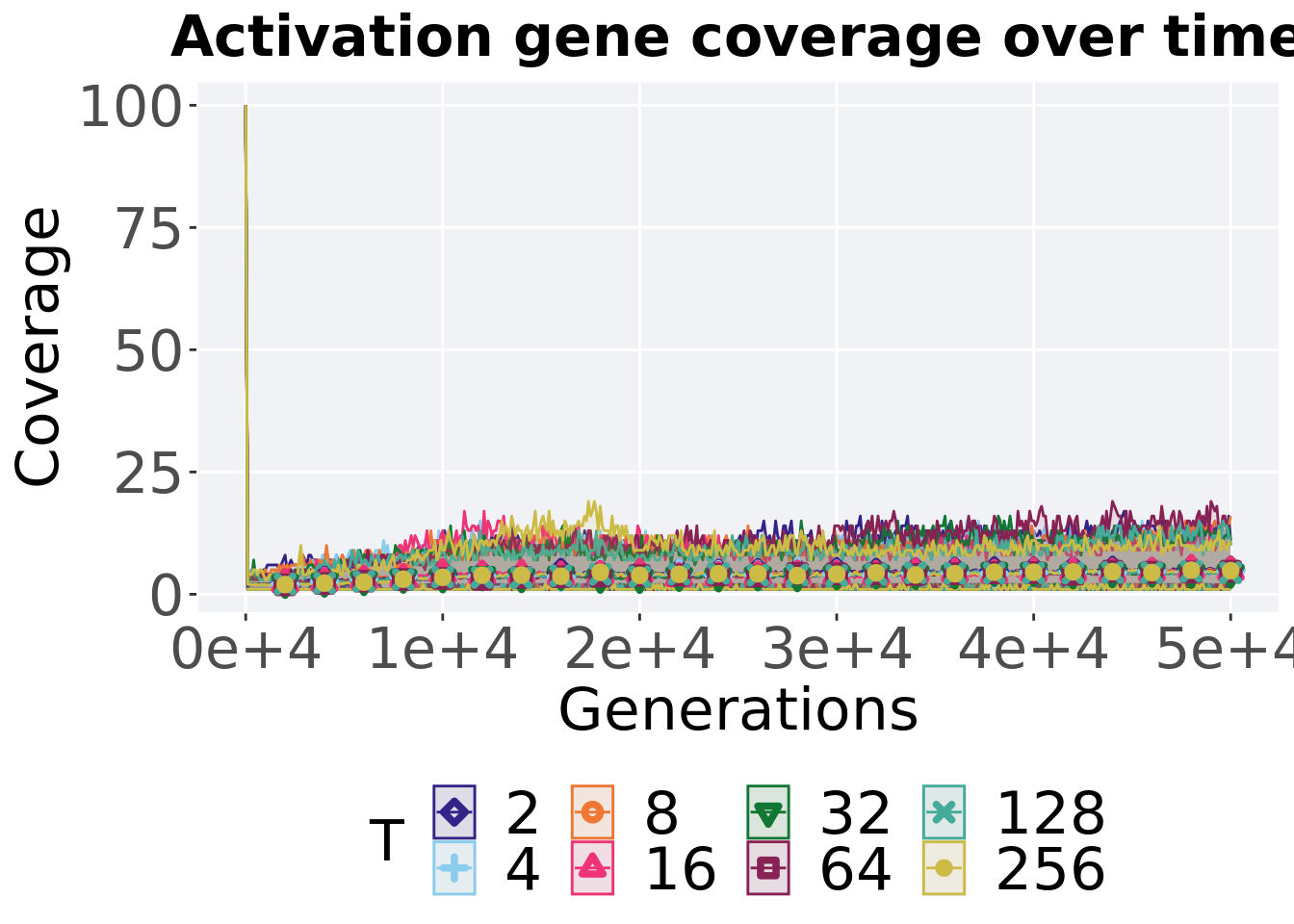

7.4.3.5 Activation gene coverage comparison

Activation gene coverage in the population at 40,000 and 50,000 generations.

# 80% and final generation comparison
end = filter(tor_ot_mvc, diagnostic == 'multipath_exploration' & gen == 50000)
end$Generation <- factor(end$gen)

mid = filter(tor_ot_mvc, diagnostic == 'multipath_exploration' & gen == 40000)
mid$Generation <- factor(mid$gen)

mvc_p = ggplot(mid, aes(x = T, y=uni_str_pos, group = T, shape = Generation)) +
  geom_point(col = mvc_col[1] , position = position_jitternudge(jitter.width = .03, nudge.x = -0.05), size = 2, alpha = 1.0) +
  geom_boxplot(position = position_nudge(x = -.15, y = 0), lwd = 0.7, col = mvc_col[1], fill = mvc_col[1], width = .1, outlier.shape = NA, alpha = 0.0) +

  geom_point(data = end, aes(x = T, y=uni_str_pos), col = mvc_col[2], position = position_jitternudge(jitter.width = .03, nudge.x = 0.05), size = 2, alpha = 1.0) +
  geom_boxplot(data = end, aes(x = T, y=uni_str_pos), position = position_nudge(x = .15, y = 0), lwd = 0.7, col = mvc_col[2], fill = mvc_col[2], width = .1, outlier.shape = NA, alpha = 0.0) +

  scale_y_continuous(
    name="Coverage",
  ) +
  scale_x_discrete(
    name="T"
  )+
  scale_shape_manual(values=c(0,1))+
  scale_colour_manual(values = c(mvc_col[1],mvc_col[2])) +
  p_theme

plot_grid(
  mvc_p +
    ggtitle("Activation gene coverage") +
    theme(legend.position="none"),
  legend,
  nrow=2,
  rel_heights = c(1,.05),
  label_size = TSIZE
)

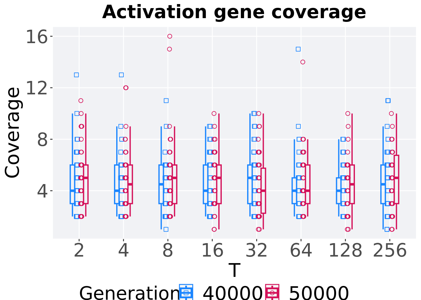
7.4.3.5.1 Stats

Summary statistics for the activation gene coverage at 40,000 and 50,000 generations.

slices = filter(tor_ot_mvc, diagnostic == 'multipath_exploration' & (gen == 50000 | gen == 40000))
slices$Generation <- factor(slices$gen, levels = c(50000,40000))
slices %>%
  group_by(T, Generation) %>%
  dplyr::summarise(
    count = n(),
    na_cnt = sum(is.na(uni_str_pos)),
    min = min(uni_str_pos, na.rm = TRUE),
    median = median(uni_str_pos, na.rm = TRUE),
    mean = mean(uni_str_pos, na.rm = TRUE),
    max = max(uni_str_pos, na.rm = TRUE),
    IQR = IQR(uni_str_pos, na.rm = TRUE)
  )

## `summarise()` has grouped output by 'T'. You can override using the `.groups`
## argument.

## # A tibble: 16 x 9
## # Groups:   T [8]
##    T     Generation count na_cnt   min median  mean   max   IQR
##    <fct> <fct>      <int>  <int> <int>  <dbl> <dbl> <int> <dbl>
##  1 2     50000         50      0     2    5    4.94    11  3   
##  2 2     40000         50      0     2    4    4.76    13  3   
##  3 4     50000         50      0     2    4.5  4.8     12  3   
##  4 4     40000         50      0     2    4    4.48    13  3   
##  5 8     50000         50      0     2    5    5.1     16  3   
##  6 8     40000         50      0     1    4.5  4.38    11  3   
##  7 16    50000         50      0     1    5    4.68    10  3   
##  8 16    40000         50      0     2    4    4.4      9  3   
##  9 32    50000         50      0     1    4    4.34    10  3.5 
## 10 32    40000         50      0     2    5    4.66    10  3   
## 11 64    50000         50      0     2    4    4.72    14  3   
## 12 64    40000         50      0     2    4    4.44    15  2   
## 13 128   50000         50      0     1    4.5  4.4     10  3   
## 14 128   40000         50      0     2    4    4.38     8  2   
## 15 256   50000         50      0     1    5    4.82    10  3.75
## 16 256   40000         50      0     1    4.5  4.5     11  3

T 2

wilcox.test(x = filter(slices, T == 2 & Generation == 50000)$uni_str_pos,
            y = filter(slices, T == 2 & Generation == 40000)$uni_str_pos,
            alternative = 't')

## 
##  Wilcoxon rank sum test with continuity correction
## 
## data:  filter(slices, T == 2 & Generation == 50000)$uni_str_pos and filter(slices, T == 2 & Generation == 40000)$uni_str_pos
## W = 1272.5, p-value = 0.878
## alternative hypothesis: true location shift is not equal to 0

T 4

wilcox.test(x = filter(slices, T == 4 & Generation == 50000)$uni_str_pos,
            y = filter(slices, T == 4 & Generation == 40000)$uni_str_pos,
            alternative = 't')

## 
##  Wilcoxon rank sum test with continuity correction
## 
## data:  filter(slices, T == 4 & Generation == 50000)$uni_str_pos and filter(slices, T == 4 & Generation == 40000)$uni_str_pos
## W = 1347.5, p-value = 0.498
## alternative hypothesis: true location shift is not equal to 0

T 8

wilcox.test(x = filter(slices, T == 8 & Generation == 50000)$uni_str_pos,
            y = filter(slices, T == 8 & Generation == 40000)$uni_str_pos,
            alternative = 't')

## 
##  Wilcoxon rank sum test with continuity correction
## 
## data:  filter(slices, T == 8 & Generation == 50000)$uni_str_pos and filter(slices, T == 8 & Generation == 40000)$uni_str_pos
## W = 1396, p-value = 0.3094
## alternative hypothesis: true location shift is not equal to 0

T 16

wilcox.test(x = filter(slices, T == 16 & Generation == 50000)$uni_str_pos,
            y = filter(slices, T == 16 & Generation == 40000)$uni_str_pos,
            alternative = 't')

## 
##  Wilcoxon rank sum test with continuity correction
## 
## data:  filter(slices, T == 16 & Generation == 50000)$uni_str_pos and filter(slices, T == 16 & Generation == 40000)$uni_str_pos
## W = 1386.5, p-value = 0.3422
## alternative hypothesis: true location shift is not equal to 0

T 32

wilcox.test(x = filter(slices, T == 32 & Generation == 50000)$uni_str_pos,
            y = filter(slices, T == 32 & Generation == 40000)$uni_str_pos,
            alternative = 't')

## 
##  Wilcoxon rank sum test with continuity correction
## 
## data:  filter(slices, T == 32 & Generation == 50000)$uni_str_pos and filter(slices, T == 32 & Generation == 40000)$uni_str_pos
## W = 1155.5, p-value = 0.5116
## alternative hypothesis: true location shift is not equal to 0

T 64

wilcox.test(x = filter(slices, T == 64 & Generation == 50000)$uni_str_pos,
            y = filter(slices, T == 64 & Generation == 40000)$uni_str_pos,
            alternative = 't')

## 
##  Wilcoxon rank sum test with continuity correction
## 
## data:  filter(slices, T == 64 & Generation == 50000)$uni_str_pos and filter(slices, T == 64 & Generation == 40000)$uni_str_pos
## W = 1346.5, p-value = 0.5018
## alternative hypothesis: true location shift is not equal to 0

T 128

wilcox.test(x = filter(slices, T == 128 & Generation == 50000)$uni_str_pos,
            y = filter(slices, T == 128 & Generation == 40000)$uni_str_pos,
            alternative = 't')

## 
##  Wilcoxon rank sum test with continuity correction
## 
## data:  filter(slices, T == 128 & Generation == 50000)$uni_str_pos and filter(slices, T == 128 & Generation == 40000)$uni_str_pos
## W = 1260.5, p-value = 0.9443
## alternative hypothesis: true location shift is not equal to 0

T 256

wilcox.test(x = filter(slices, T == 256 & Generation == 50000)$uni_str_pos,
            y = filter(slices, T == 256 & Generation == 40000)$uni_str_pos,
            alternative = 't')

## 
##  Wilcoxon rank sum test with continuity correction
## 
## data:  filter(slices, T == 256 & Generation == 50000)$uni_str_pos and filter(slices, T == 256 & Generation == 40000)$uni_str_pos
## W = 1377.5, p-value = 0.3761
## alternative hypothesis: true location shift is not equal to 0