Chapter 5 Multi-path mpeloration results

Here we present the results for the best performances and activation gene coverage generated by each selection scheme replicate on the multi-path mpeloration diagnostic. Best performance found refers to the largest average trait score found in a given population. Note that activation gene coverage values are gathered at the population-level. Activation gene coverage refers to the count of unique activation genes in a given population; this gives us a range of integers between 0 and 100.

5.1 Analysis dependencies

library(ggplot2)
library(cowplot)
library(dplyr)
library(PupillometryR)
library(sdamr)

5.2 Performance

Performance analysis.

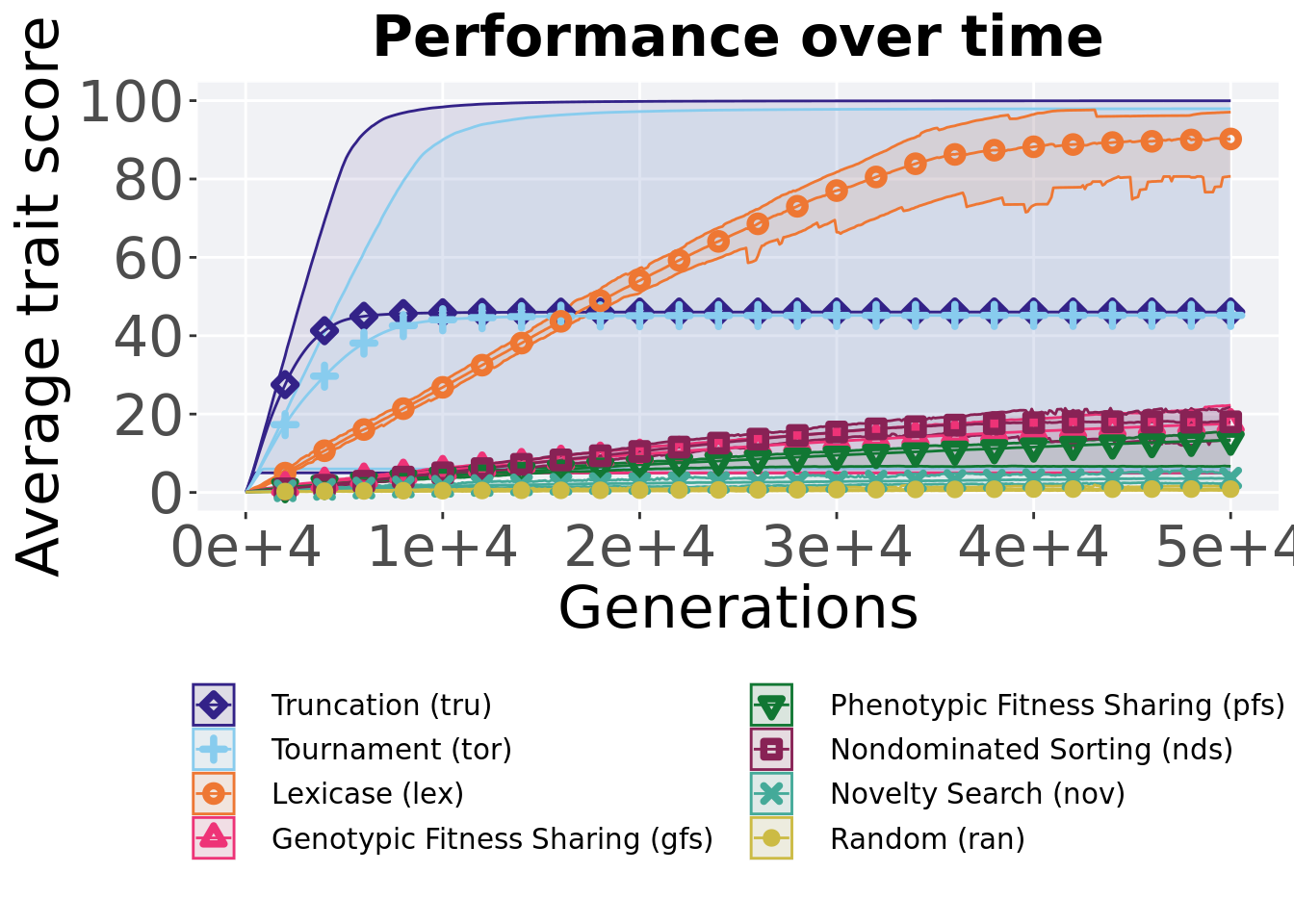
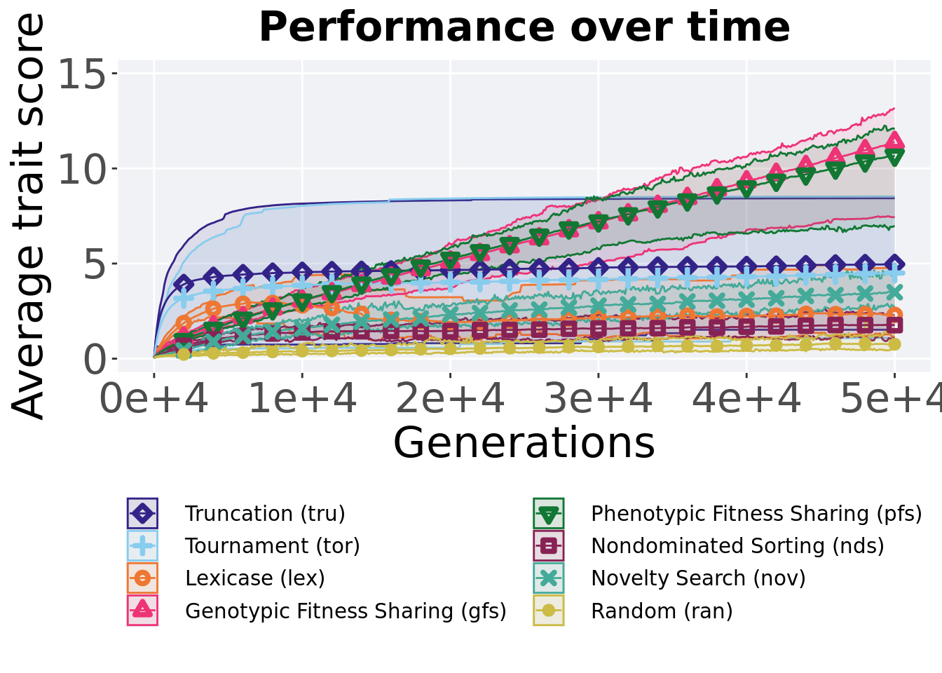
5.2.1 Over time

Best performance in a population over time.

# data for lines and shading on plots
lines = filter(cc_over_time, diagnostic == 'multipath_exploration') %>%
  group_by(`Selection\nScheme`, gen) %>%
  dplyr::summarise(
    min = min(pop_fit_max) / DIMENSIONALITY,
    mean = mean(pop_fit_max) / DIMENSIONALITY,
    max = max(pop_fit_max) / DIMENSIONALITY
  )

## `summarise()` has grouped output by 'Selection Scheme'. You can override using
## the `.groups` argument.

ggplot(lines, aes(x=gen, y=mean, group = `Selection\nScheme`, fill =`Selection\nScheme`, color = `Selection\nScheme`, shape = `Selection\nScheme`)) +
  geom_ribbon(aes(ymin = min, ymax = max), alpha = 0.1) +
  geom_line(size = 0.5) +
  geom_point(data = filter(lines, gen %% 2000 == 0 & gen != 0), size = 1.5, stroke = 2.0, alpha = 1.0) +
  scale_y_continuous(
    name="Average trait score",
    limits=c(0, 100),
    breaks=seq(0,100, 20),
    labels=c("0", "20", "40", "60", "80", "100")
  ) +
  scale_x_continuous(
    name="Generations",
    limits=c(0, 50000),
    breaks=c(0, 10000, 20000, 30000, 40000, 50000),
    labels=c("0e+4", "1e+4", "2e+4", "3e+4", "4e+4", "5e+4")

  ) +
  scale_shape_manual(values=SHAPE)+
  scale_colour_manual(values = cb_palette) +
  scale_fill_manual(values = cb_palette) +
  ggtitle('Performance over time')+
  p_theme + theme(legend.title=element_blank(),legend.text=element_text(size=11)) +
  guides(
    shape=guide_legend(ncol=2, title.position = "bottom"),
    color=guide_legend(ncol=2, title.position = "bottom"),
    fill=guide_legend(ncol=2, title.position = "bottom")
  )

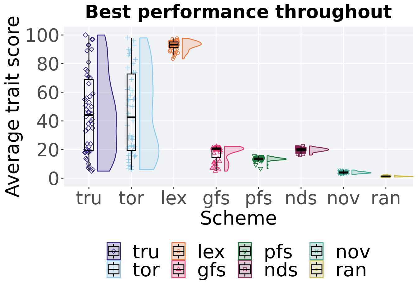
5.2.2 Best performance throughout

Best performance throughout 50,000 generations.

### best performance throughout
filter(cc_best, col == 'pop_fit_max' & diagnostic == 'multipath_exploration') %>%
  ggplot(., aes(x = acron, y = val / DIMENSIONALITY, color = acron, fill = acron, shape = acron)) +
  geom_flat_violin(position = position_nudge(x = .2, y = 0), scale = 'width', alpha = 0.2) +
  geom_point(position = position_jitter(width = .1), size = 1.5, alpha = 1.0) +
  geom_boxplot(color = 'black', width = .2, outlier.shape = NA, alpha = 0.0) +
  guides(fill = "none",color = 'none', shape = 'none') +
  scale_y_continuous(
    name="Average trait score",
    limits=c(-1, 101),
    breaks=seq(0,100, 20),
    labels=c("0", "20", "40", "60", "80", "100")
  ) +
  scale_x_discrete(
    name="Scheme"
  )+
  scale_shape_manual(values=SHAPE)+
  scale_colour_manual(values = cb_palette, ) +
  scale_fill_manual(values = cb_palette) +
  ggtitle('Best performance throughout')+
  p_theme + theme(legend.title=element_blank()) +
  guides(
    shape=guide_legend(nrow=2, title.position = "bottom"),
    color=guide_legend(nrow=2, title.position = "bottom"),
    fill=guide_legend(nrow=2, title.position = "bottom")
  )

5.2.2.1 Stats

Summary statistics for the best performance.

### best performance throughout
performance = filter(cc_best, col == 'pop_fit_max' & diagnostic == 'multipath_exploration')
performance$acron = factor(performance$acron, levels = c('lex','tor','tru','nds','gfs','pfs','nov','ran'))
performance %>%
  group_by(acron) %>%
  dplyr::summarise(
    count = n(),
    na_cnt = sum(is.na(val)),
    min = min(val / DIMENSIONALITY, na.rm = TRUE),
    median = median(val / DIMENSIONALITY, na.rm = TRUE),
    mean = mean(val / DIMENSIONALITY, na.rm = TRUE),
    max = max(val / DIMENSIONALITY, na.rm = TRUE),
    IQR = IQR(val / DIMENSIONALITY, na.rm = TRUE)
  )

## # A tibble: 8 x 8
##   acron count na_cnt    min median  mean    max    IQR
##   <fct> <int>  <int>  <dbl>  <dbl> <dbl>  <dbl>  <dbl>
## 1 lex      50      0 83.4    93.2  92.5   97.7   4.05 
## 2 tor      50      0  6.00   42.5  45.2   97.9  53.2  
## 3 tru      50      0  5      44.0  46.1  100.   49.7  
## 4 nds      50      0 16.2    19.9  19.8   22.5   1.59 
## 5 gfs      50      0  4.99   20.4  17.6   22.2   6.69 
## 6 pfs      50      0  6.76   13.5  13.4   15.6   1.10 
## 7 nov      50      0  2.62    3.89  4.01   5.68  0.860
## 8 ran      50      0  0.870   1.25  1.28   2.04  0.288

Kruskal–Wallis test provides evidence of difference among best performances.

kruskal.test(val ~ acron, data = performance)

## 
##  Kruskal-Wallis rank sum test
## 
## data:  val by acron
## Kruskal-Wallis chi-squared = 329.88, df = 7, p-value < 2.2e-16

Results for post-hoc Wilcoxon rank-sum test with a Bonferroni correction on best performance.

pairwise.wilcox.test(x = performance$val, g = performance$acron, p.adjust.method = "bonferroni",
                     paired = FALSE, conf.int = FALSE, alternative = 'l')

## 
##  Pairwise comparisons using Wilcoxon rank sum test with continuity correction 
## 
## data:  performance$val and performance$acron 
## 
##     lex     tor     tru     nds     gfs     pfs     nov    
## tor 3.0e-13 -       -       -       -       -       -      
## tru 1.1e-11 1.00000 -       -       -       -       -      
## nds < 2e-16 0.00047 0.00027 -       -       -       -      
## gfs < 2e-16 2.3e-05 1.6e-05 1.00000 -       -       -      
## pfs < 2e-16 3.1e-08 6.9e-10 < 2e-16 0.00015 -       -      
## nov < 2e-16 < 2e-16 < 2e-16 < 2e-16 < 2e-16 < 2e-16 -      
## ran < 2e-16 < 2e-16 < 2e-16 < 2e-16 < 2e-16 < 2e-16 < 2e-16
## 
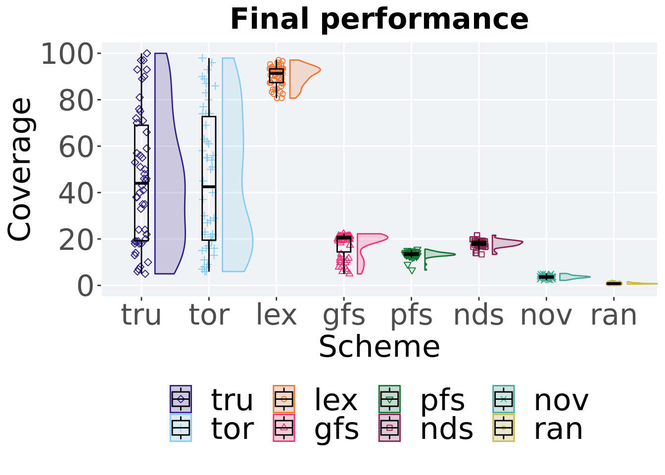
## P value adjustment method: bonferroni

5.2.3 End of 50,000 generations

Best performance in the population at the end of 50,000 generations.

# end of run
filter(cc_over_time, diagnostic == 'multipath_exploration' & gen == 50000) %>%
  ggplot(., aes(x = acron, y = pop_fit_max / DIMENSIONALITY, color = acron, fill = acron, shape = acron)) +
  geom_flat_violin(position = position_nudge(x = .2, y = 0), scale = 'width', alpha = 0.2) +
  geom_point(position = position_jitter(width = .1), size = 1.5, alpha = 1.0) +
  geom_boxplot(color = 'black', width = .2, outlier.shape = NA, alpha = 0.0) +
  guides(fill = "none",color = 'none', shape = 'none') +
  scale_y_continuous(
    name="Coverage",
    limits=c(0, 100),
    breaks=seq(0,100, 20),
    labels=c("0", "20", "40", "60", "80", "100")
  ) +
  scale_x_discrete(
    name="Scheme"
  )+
  scale_shape_manual(values=SHAPE)+
  scale_colour_manual(values = cb_palette, ) +
  scale_fill_manual(values = cb_palette) +
  ggtitle('Final performance')+
  p_theme + theme(legend.title=element_blank()) +
  guides(
    shape=guide_legend(nrow=2, title.position = "bottom"),
    color=guide_legend(nrow=2, title.position = "bottom"),
    fill=guide_legend(nrow=2, title.position = "bottom")
  )

5.2.3.1 Stats

Summary statistics for best performance in the final population.

# end of run
performance = filter(cc_over_time, diagnostic == 'multipath_exploration' & gen == 50000)
performance$acron = factor(performance$acron, levels = c('lex','tor','tru','nds','gfs','pfs','nov','ran'))
performance %>%
  group_by(acron) %>%
  dplyr::summarise(
    count = n(),
    na_cnt = sum(is.na(pop_fit_max / DIMENSIONALITY)),
    min = min(pop_fit_max / DIMENSIONALITY, na.rm = TRUE),
    median = median(pop_fit_max / DIMENSIONALITY, na.rm = TRUE),
    mean = mean(pop_fit_max / DIMENSIONALITY, na.rm = TRUE),
    max = max(pop_fit_max / DIMENSIONALITY, na.rm = TRUE),
    IQR = IQR(pop_fit_max / DIMENSIONALITY, na.rm = TRUE)
  )

## # A tibble: 8 x 8
##   acron count na_cnt    min median   mean    max    IQR
##   <fct> <int>  <int>  <dbl>  <dbl>  <dbl>  <dbl>  <dbl>
## 1 lex      50      0 80.7   91.3   90.2    97.1   5.91 
## 2 tor      50      0  6.00  42.5   45.2    97.9  53.2  
## 3 tru      50      0  5     44.0   46.1   100.   49.7  
## 4 nds      50      0 13.4   18.1   18.0    21.6   1.65 
## 5 gfs      50      0  4.96  20.4   17.6    22.2   6.68 
## 6 pfs      50      0  6.67  13.5   13.3    15.6   1.04 
## 7 nov      50      0  2.16   3.66   3.64    5.12  0.859
## 8 ran      50      0  0.553  0.785  0.840   1.56  0.299

Kruskal–Wallis test provides evidence of difference among best performance in the final population.

kruskal.test(pop_fit_max ~ acron, data = performance)

## 
##  Kruskal-Wallis rank sum test
## 
## data:  pop_fit_max by acron
## Kruskal-Wallis chi-squared = 330.05, df = 7, p-value < 2.2e-16

Results for post-hoc Wilcoxon rank-sum test with a Bonferroni correction on best performance in the final population.

pairwise.wilcox.test(x = performance$pop_fit_max, g = performance$acron, p.adjust.method = "bonferroni",
                     paired = FALSE, conf.int = FALSE, alternative = 'l')

## 
##  Pairwise comparisons using Wilcoxon rank sum test with continuity correction 
## 
## data:  performance$pop_fit_max and performance$acron 
## 
##     lex     tor     tru     nds     gfs     pfs     nov    
## tor 3.9e-12 -       -       -       -       -       -      
## tru 7.1e-11 1.00000 -       -       -       -       -      
## nds < 2e-16 8.2e-05 9.3e-07 -       -       -       -      
## gfs < 2e-16 2.2e-05 1.6e-05 1.00000 -       -       -      
## pfs < 2e-16 3.0e-08 6.6e-10 3.0e-15 0.00015 -       -      
## nov < 2e-16 < 2e-16 < 2e-16 < 2e-16 < 2e-16 < 2e-16 -      
## ran < 2e-16 < 2e-16 < 2e-16 < 2e-16 < 2e-16 < 2e-16 < 2e-16
## 
## P value adjustment method: bonferroni

5.3 Activation gene coverage

Activation gene coverage analysis.

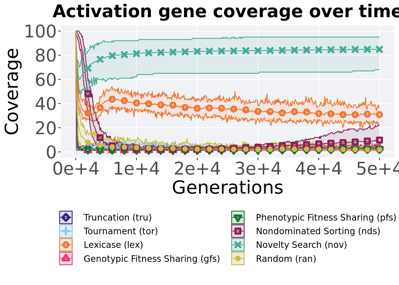
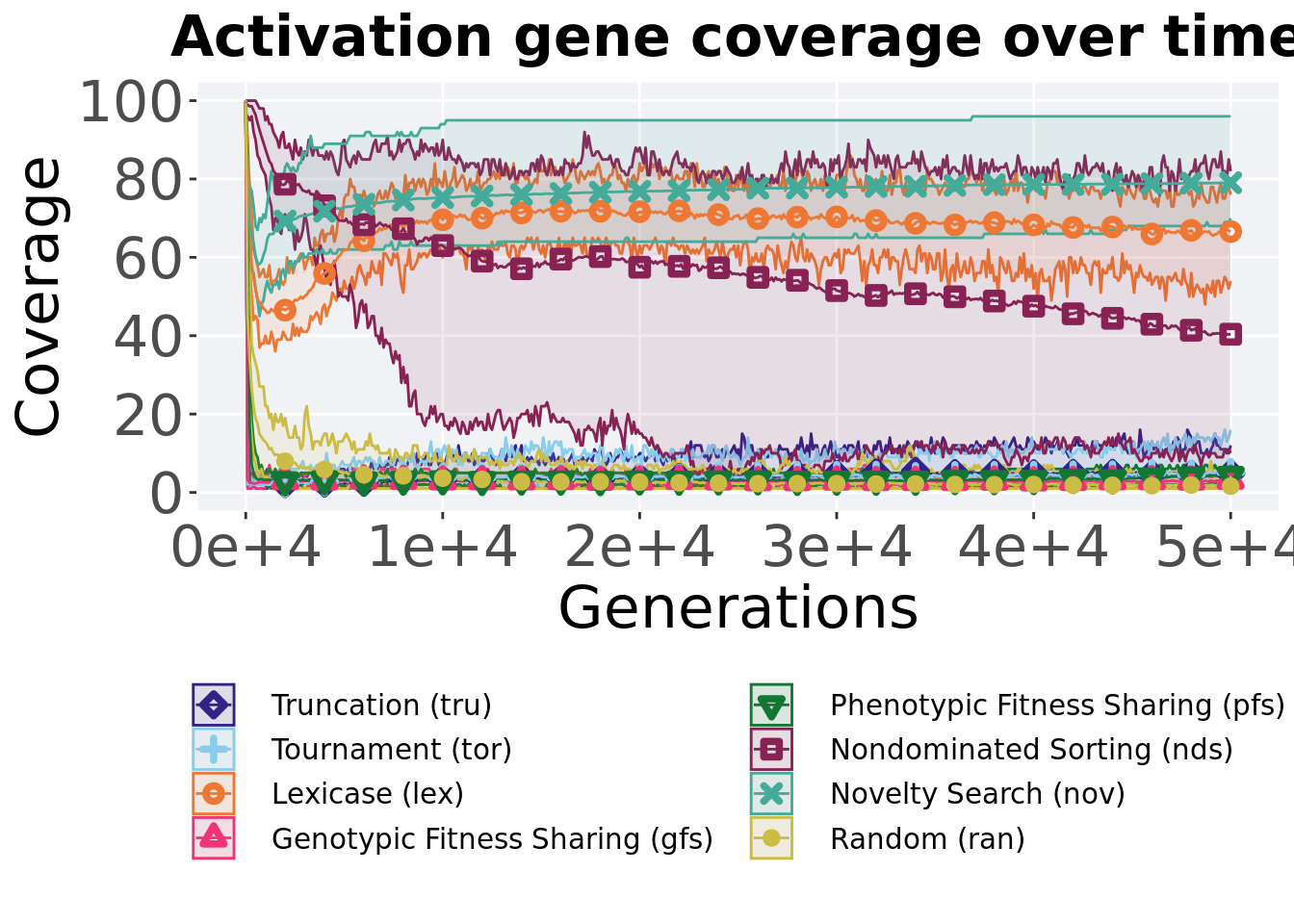
5.3.1 Over time coverage

Activation gene coverage over time.

# data for lines and shading on plots
lines = filter(cc_over_time, diagnostic == 'multipath_exploration') %>%
  group_by(`Selection\nScheme`, gen) %>%
  dplyr::summarise(
    min = min(uni_str_pos),
    mean = mean(uni_str_pos),
    max = max(uni_str_pos)
  )

## `summarise()` has grouped output by 'Selection Scheme'. You can override using
## the `.groups` argument.

ggplot(lines, aes(x=gen, y=mean, group = `Selection\nScheme`, fill =`Selection\nScheme`, color = `Selection\nScheme`, shape = `Selection\nScheme`)) +
  geom_ribbon(aes(ymin = min, ymax = max), alpha = 0.1) +
  geom_line(size = 0.5) +
  geom_point(data = filter(lines, gen %% 2000 == 0 & gen != 0), size = 1.5, stroke = 2.0, alpha = 1.0) +
  scale_y_continuous(
    name="Coverage",
    limits=c(0, 100),
    breaks=seq(0,100, 20),
    labels=c("0", "20", "40", "60", "80", "100")
  ) +
  scale_x_continuous(
    name="Generations",
    limits=c(0, 50000),
    breaks=c(0, 10000, 20000, 30000, 40000, 50000),
    labels=c("0e+4", "1e+4", "2e+4", "3e+4", "4e+4", "5e+4")
  ) +
  scale_shape_manual(values=SHAPE)+
  scale_colour_manual(values = cb_palette) +
  scale_fill_manual(values = cb_palette) +
  ggtitle('Activation gene coverage over time')+
  p_theme + theme(legend.title=element_blank(),legend.text=element_text(size=11)) +
  guides(
    shape=guide_legend(ncol=2, title.position = "bottom"),
    color=guide_legend(ncol=2, title.position = "bottom"),
    fill=guide_legend(ncol=2, title.position = "bottom")
  )

5.3.2 End of 50,000 generations

Activation gene coverage in the population at the end of 50,000 generations.

# end of run
filter(cc_over_time, diagnostic == 'multipath_exploration' & gen == 50000) %>%
  ggplot(., aes(x = acron, y = uni_str_pos, color = acron, fill = acron, shape = acron)) +
  geom_flat_violin(position = position_nudge(x = .2, y = 0), scale = 'width', alpha = 0.2) +
  geom_point(position = position_jitter(width = .1), size = 1.5, alpha = 1.0) +
  geom_boxplot(color = 'black', width = .2, outlier.shape = NA, alpha = 0.0) +
  guides(fill = "none",color = 'none', shape = 'none') +
  scale_y_continuous(
    name="Coverage",
    limits=c(0, 100),
    breaks=seq(0,100, 20),
    labels=c("0", "20", "40", "60", "80", "100")
  ) +
  scale_x_discrete(
    name="Scheme"
  )+
  scale_shape_manual(values=SHAPE)+
  scale_colour_manual(values = cb_palette, ) +
  scale_fill_manual(values = cb_palette) +
  ggtitle('Final activation gene coverage')+
  p_theme + theme(legend.title=element_blank()) +
  guides(
    shape=guide_legend(nrow=2, title.position = "bottom"),
    color=guide_legend(nrow=2, title.position = "bottom"),
    fill=guide_legend(nrow=2, title.position = "bottom")
  )

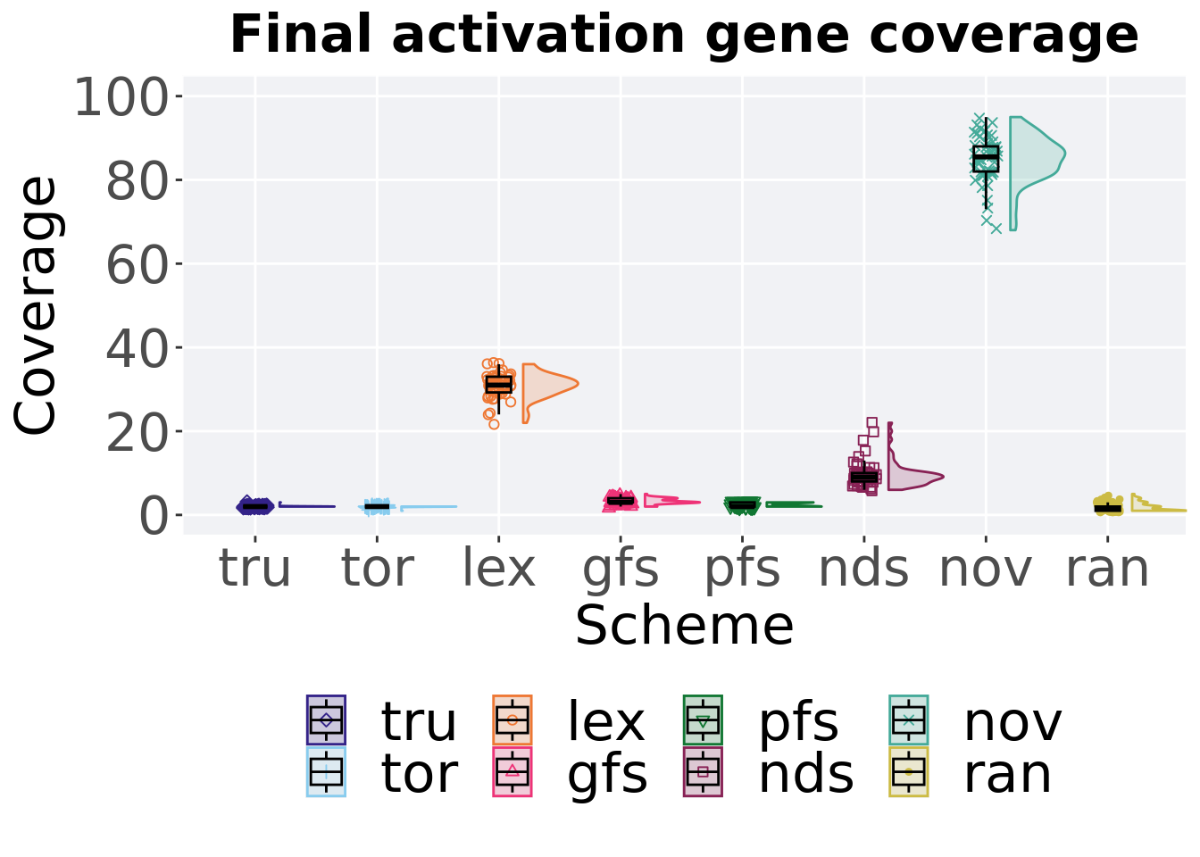
5.3.2.1 Stats

Summary statistics for activation gene coverage in the final population.

# end of run
coverage = filter(cc_over_time, diagnostic == 'multipath_exploration' & gen == 50000)
coverage$acron = factor(coverage$acron, levels = c('nov','lex','nds','gfs','pfs','tor','tru','ran'))
coverage %>%
  group_by(acron) %>%
  dplyr::summarise(
    count = n(),
    na_cnt = sum(is.na(uni_str_pos)),
    min = min(uni_str_pos, na.rm = TRUE),
    median = median(uni_str_pos, na.rm = TRUE),
    mean = mean(uni_str_pos, na.rm = TRUE),
    max = max(uni_str_pos, na.rm = TRUE),
    IQR = IQR(uni_str_pos, na.rm = TRUE)
  )

## # A tibble: 8 x 8
##   acron count na_cnt   min median  mean   max   IQR
##   <fct> <int>  <int> <int>  <dbl> <dbl> <int> <dbl>
## 1 nov      50      0    68   85.5 84.9     95  6   
## 2 lex      50      0    22   31   30.8     36  3.75
## 3 nds      50      0     6    9    9.76    22  2   
## 4 gfs      50      0     2    3    3.24     5  1   
## 5 pfs      50      0     2    2    2.46     3  1   
## 6 tor      50      0     1    2    1.98     2  0   
## 7 tru      50      0     2    2    2.02     3  0   
## 8 ran      50      0     1    1.5  1.86     5  1

Kruskal–Wallis test provides evidence of difference among activation gene coverage in the final population.

kruskal.test(uni_str_pos ~ acron, data = coverage)

## 
##  Kruskal-Wallis rank sum test
## 
## data:  uni_str_pos by acron
## Kruskal-Wallis chi-squared = 351.29, df = 7, p-value < 2.2e-16

Results for post-hoc Wilcoxon rank-sum test with a Bonferroni correction on activation gene coverage in the final population.

pairwise.wilcox.test(x = coverage$uni_str_pos, g = coverage$acron, p.adjust.method = "bonferroni",
                     paired = FALSE, conf.int = FALSE, alternative = 'l')

## 
##  Pairwise comparisons using Wilcoxon rank sum test with continuity correction 
## 
## data:  coverage$uni_str_pos and coverage$acron 
## 
##     nov     lex     nds     gfs     pfs     tor     tru    
## lex < 2e-16 -       -       -       -       -       -      
## nds < 2e-16 < 2e-16 -       -       -       -       -      
## gfs < 2e-16 < 2e-16 < 2e-16 -       -       -       -      
## pfs < 2e-16 < 2e-16 < 2e-16 7.8e-07 -       -       -      
## tor < 2e-16 < 2e-16 < 2e-16 4.2e-16 6.3e-07 -       -      
## tru < 2e-16 < 2e-16 < 2e-16 1.4e-15 4.3e-06 1.00000 -      
## ran < 2e-16 < 2e-16 < 2e-16 1.1e-08 0.00073 0.20446 0.10598
## 
## P value adjustment method: bonferroni

5.4 Multi-valley crossing results

5.4.1 Performance

Performance analysis.

5.4.1.1 Performance over time

Best performance in a population over time.

# data for lines and shading on plots
lines = filter(cc_over_time_mvc, diagnostic == 'multipath_exploration') %>%
  group_by(`Selection\nScheme`, gen) %>%
  dplyr::summarise(
    min = min(pop_fit_max) / DIMENSIONALITY,
    mean = mean(pop_fit_max) / DIMENSIONALITY,
    max = max(pop_fit_max) / DIMENSIONALITY
  )

## `summarise()` has grouped output by 'Selection Scheme'. You can override using
## the `.groups` argument.

ggplot(lines, aes(x=gen, y=mean, group = `Selection\nScheme`, fill =`Selection\nScheme`, color = `Selection\nScheme`, shape = `Selection\nScheme`)) +
  geom_ribbon(aes(ymin = min, ymax = max), alpha = 0.1) +
  geom_line(size = 0.5) +
  geom_point(data = filter(lines, gen %% 2000 == 0 & gen != 0), size = 1.5, stroke = 2.0, alpha = 1.0) +
  scale_y_continuous(
    name="Average trait score",
    limits=c(0, 15),
    breaks=seq(0,15, 5),
    labels=c("0", "5", "10", "15")
  ) +
  scale_x_continuous(
    name="Generations",
    limits=c(0, 50000),
    breaks=c(0, 10000, 20000, 30000, 40000, 50000),
    labels=c("0e+4", "1e+4", "2e+4", "3e+4", "4e+4", "5e+4")

  ) +
  scale_shape_manual(values=SHAPE)+
  scale_colour_manual(values = cb_palette) +
  scale_fill_manual(values = cb_palette) +
  ggtitle('Performance over time')+
  p_theme + theme(legend.title=element_blank(),legend.text=element_text(size=11)) +
  guides(
    shape=guide_legend(ncol=2, title.position = "bottom"),
    color=guide_legend(ncol=2, title.position = "bottom"),
    fill=guide_legend(ncol=2, title.position = "bottom")
  )

5.4.1.2 Best performance throughout

Best performance found throughout 50,000 generations.

### best performance throughout
filter(cc_best_mvc, col == 'pop_fit_max' & diagnostic == 'multipath_exploration') %>%
  ggplot(., aes(x = acron, y = val / DIMENSIONALITY, color = acron, fill = acron, shape = acron)) +
  geom_flat_violin(position = position_nudge(x = .2, y = 0), scale = 'width', alpha = 0.2) +
  geom_point(position = position_jitter(width = .1), size = 1.5, alpha = 1.0) +
  geom_boxplot(color = 'black', width = .2, outlier.shape = NA, alpha = 0.0) +
  guides(fill = "none",color = 'none', shape = 'none') +
  scale_y_continuous(
    name="Average trait score",
    limits=c(0, 15),
    breaks=seq(0,15, 5),
    labels=c("0", "5", "10", "15")
  ) +
  scale_x_discrete(
    name="Scheme"
  )+
  scale_shape_manual(values=SHAPE)+
  scale_colour_manual(values = cb_palette, ) +
  scale_fill_manual(values = cb_palette) +
  ggtitle('Best performance throughout')+
  p_theme + theme(legend.title=element_blank()) +
  guides(
    shape=guide_legend(nrow=2, title.position = "bottom"),
    color=guide_legend(nrow=2, title.position = "bottom"),
    fill=guide_legend(nrow=2, title.position = "bottom")
  )

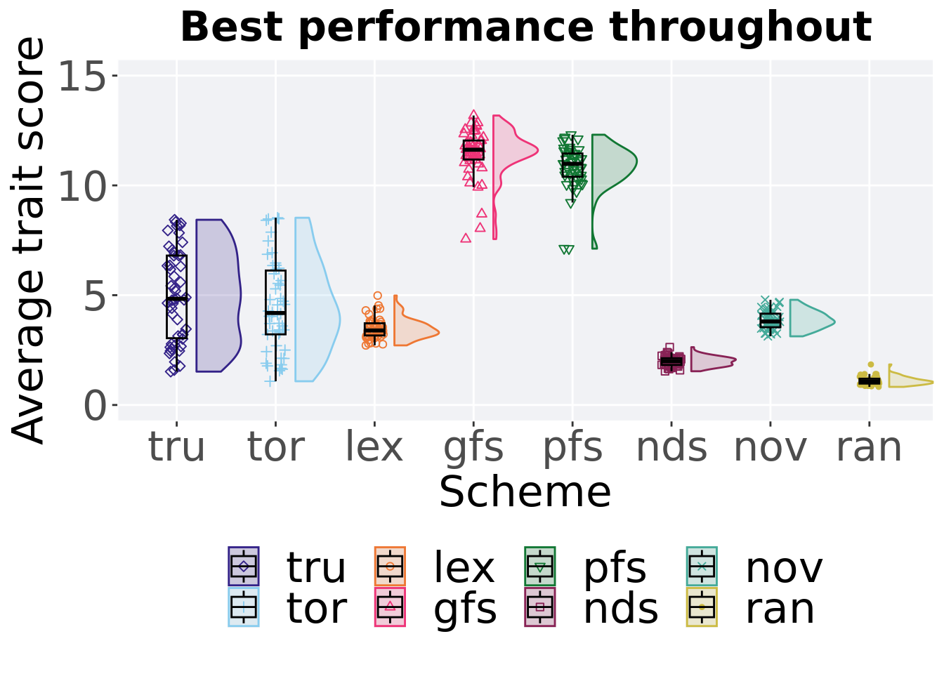
5.4.1.2.1 Stats

Summary statistics for the performance of the best performance.

### best performance throughout
performance = filter(cc_best_mvc, col == 'pop_fit_max' & diagnostic == 'multipath_exploration')
performance$acron = factor(performance$acron, levels = c('gfs','pfs','tor','tru','nov','lex','nds','ran'))
performance %>%
  group_by(acron) %>%
  dplyr::summarise(
    count = n(),
    na_cnt = sum(is.na(val)),
    min = min(val / DIMENSIONALITY, na.rm = TRUE),
    median = median(val / DIMENSIONALITY, na.rm = TRUE),
    mean = mean(val / DIMENSIONALITY, na.rm = TRUE),
    max = max(val / DIMENSIONALITY, na.rm = TRUE),
    IQR = IQR(val / DIMENSIONALITY, na.rm = TRUE)
  )

## # A tibble: 8 x 8
##   acron count na_cnt   min median  mean   max   IQR
##   <fct> <int>  <int> <dbl>  <dbl> <dbl> <dbl> <dbl>
## 1 gfs      50      0 7.56   11.6  11.5  13.2  0.865
## 2 pfs      50      0 7.12   11.0  10.8  12.3  1.06 
## 3 tor      50      0 1.08    4.19  4.50  8.53 2.91 
## 4 tru      50      0 1.52    4.83  4.96  8.43 3.76 
## 5 nov      50      0 3.13    3.80  3.88  4.79 0.617
## 6 lex      50      0 2.71    3.39  3.48  4.98 0.555
## 7 nds      50      0 1.54    1.99  1.98  2.63 0.307
## 8 ran      50      0 0.825   1.07  1.10  1.85 0.222

Kruskal–Wallis test provides evidence of statistical differences.

kruskal.test(val ~ acron, data = performance)

## 
##  Kruskal-Wallis rank sum test
## 
## data:  val by acron
## Kruskal-Wallis chi-squared = 335.6, df = 7, p-value < 2.2e-16

Results for post-hoc Wilcoxon rank-sum test with a Bonferroni correction.

pairwise.wilcox.test(x = performance$val, g = performance$acron, p.adjust.method = "bonferroni",
                     paired = FALSE, conf.int = FALSE, alternative = 'l')

## 
##  Pairwise comparisons using Wilcoxon rank sum test with continuity correction 
## 
## data:  performance$val and performance$acron 
## 
##     gfs     pfs     tor     tru     nov     lex     nds    
## pfs 0.00212 -       -       -       -       -       -      
## tor < 2e-16 < 2e-16 -       -       -       -       -      
## tru < 2e-16 2.9e-16 1.00000 -       -       -       -      
## nov < 2e-16 < 2e-16 1.00000 0.18480 -       -       -      
## lex < 2e-16 < 2e-16 0.08240 0.02364 0.00014 -       -      
## nds < 2e-16 < 2e-16 2.5e-09 1.7e-12 < 2e-16 < 2e-16 -      
## ran < 2e-16 < 2e-16 5.2e-16 < 2e-16 < 2e-16 < 2e-16 2.6e-16
## 
## P value adjustment method: bonferroni

5.4.1.3 Performance comparison

Best performances in the population at 40,000 and 50,000 generations.

## Warning: The following aesthetics were dropped during statistical transformation:
## colour, shape
## i This can happen when ggplot fails to infer the correct grouping structure in
##   the data.
## i Did you forget to specify a `group` aesthetic or to convert a numerical
##   variable into a factor?
## The following aesthetics were dropped during statistical transformation:
## colour, shape
## i This can happen when ggplot fails to infer the correct grouping structure in
##   the data.
## i Did you forget to specify a `group` aesthetic or to convert a numerical
##   variable into a factor?

# 80% and final generation comparison
end = filter(cc_over_time_mvc, diagnostic == 'multipath_exploration' & gen == 50000 & acron != 'ran')
end$Generation <- factor(end$gen)

mid = filter(cc_over_time_mvc, diagnostic == 'multipath_exploration' & gen == 40000 & acron != 'ran')
mid$Generation <- factor(mid$gen)

mvc_p = ggplot(mid, aes(x = acron, y=pop_fit_max / DIMENSIONALITY, group = acron, shape = Generation)) +
  geom_point(col = mvc_col[1] , position = position_jitternudge(jitter.width = .03, nudge.x = -0.05), size = 2, alpha = 1.0) +
  geom_boxplot(position = position_nudge(x = -.15, y = 0), lwd = 0.7, col = mvc_col[1], fill = mvc_col[1], width = .1, outlier.shape = NA, alpha = 0.0) +

  geom_point(data = end, aes(x = acron, y=pop_fit_max / DIMENSIONALITY), col = mvc_col[2], position = position_jitternudge(jitter.width = .03, nudge.x = 0.05), size = 2, alpha = 1.0) +
  geom_boxplot(data = end, aes(x = acron, y=pop_fit_max / DIMENSIONALITY), position = position_nudge(x = .15, y = 0), lwd = 0.7, col = mvc_col[2], fill = mvc_col[2], width = .1, outlier.shape = NA, alpha = 0.0) +

  scale_y_continuous(
    name="Average trait score",
    limits=c(0, 15),
    breaks=seq(0,15, 5),
    labels=c("0", "5", "10", "15")
  ) +
  scale_x_discrete(
    name="Scheme"
  )+
  scale_shape_manual(values=c(0,1))+
  scale_colour_manual(values = c(mvc_col[1],mvc_col[2])) +
  p_theme

plot_grid(
  mvc_p +
    ggtitle("Performance comparisons") +
    theme(legend.position="none"),
  legend,
  nrow=2,
  rel_heights = c(1,.05),
  label_size = TSIZE
)

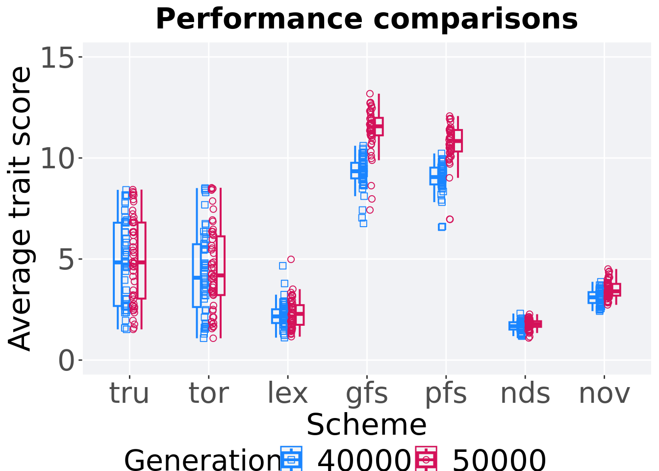
5.4.1.3.1 Stats

Summary statistics for the performance of the best performance at 40,000 and 50,000 generations.

### performance comparisons and generation slices 40K & 50K
slices = filter(cc_over_time_mvc, diagnostic == 'multipath_exploration' & (gen == 50000 | gen == 40000) & acron != 'ran')
slices$Generation <- factor(slices$gen, levels = c(50000,40000))
slices$acron = factor(slices$acron, levels = c('gfs','pfs','tru','tor','nov', 'nds','lex', 'ran'))
slices %>%
  group_by(acron, Generation) %>%
  dplyr::summarise(
    count = n(),
    na_cnt = sum(is.na(pop_fit_max  / DIMENSIONALITY)),
    min = min(pop_fit_max  / DIMENSIONALITY, na.rm = TRUE),
    median = median(pop_fit_max  / DIMENSIONALITY, na.rm = TRUE),
    mean = mean(pop_fit_max  / DIMENSIONALITY, na.rm = TRUE),
    max = max(pop_fit_max  / DIMENSIONALITY, na.rm = TRUE),
    IQR = IQR(pop_fit_max  / DIMENSIONALITY, na.rm = TRUE)
  )

## `summarise()` has grouped output by 'acron'. You can override using the
## `.groups` argument.

## # A tibble: 14 x 9
## # Groups:   acron [7]
##    acron Generation count na_cnt   min median  mean   max   IQR
##    <fct> <fct>      <int>  <int> <dbl>  <dbl> <dbl> <dbl> <dbl>
##  1 gfs   50000         50      0  7.43  11.6  11.4  13.2  0.865
##  2 gfs   40000         50      0  6.76   9.34  9.32 10.6  0.772
##  3 pfs   50000         50      0  6.96  10.8  10.7  12.1  1.06 
##  4 pfs   40000         50      0  6.57   9.06  9.01 10.2  0.832
##  5 tru   50000         50      0  1.52   4.83  4.96  8.43 3.76 
##  6 tru   40000         50      0  1.52   4.83  4.85  8.42 4.12 
##  7 tor   50000         50      0  1.08   4.19  4.50  8.53 2.91 
##  8 tor   40000         50      0  1.08   4.07  4.31  8.51 3.11 
##  9 nov   50000         50      0  2.73   3.40  3.49  4.51 0.582
## 10 nov   40000         50      0  2.42   3.11  3.10  3.87 0.538
## 11 nds   50000         50      0  1.09   1.78  1.76  2.27 0.279
## 12 nds   40000         50      0  1.19   1.68  1.68  2.30 0.363
## 13 lex   50000         50      0  1.16   2.29  2.30  4.98 0.974
## 14 lex   40000         50      0  1.11   2.16  2.25  4.67 0.681

Truncation selection comparisons.

wilcox.test(x = filter(slices, acron == 'tru' & Generation == 50000)$pop_fit_max,
            y = filter(slices, acron == 'tru' & Generation == 40000)$pop_fit_max,
            alternative = 't')

## 
##  Wilcoxon rank sum test with continuity correction
## 
## data:  filter(slices, acron == "tru" & Generation == 50000)$pop_fit_max and filter(slices, acron == "tru" & Generation == 40000)$pop_fit_max
## W = 1317, p-value = 0.6466
## alternative hypothesis: true location shift is not equal to 0

Tournament selection comparisons.

wilcox.test(x = filter(slices, acron == 'tor' & Generation == 50000)$pop_fit_max,
            y = filter(slices, acron == 'tor' & Generation == 40000)$pop_fit_max,
            alternative = 't')

## 
##  Wilcoxon rank sum test with continuity correction
## 
## data:  filter(slices, acron == "tor" & Generation == 50000)$pop_fit_max and filter(slices, acron == "tor" & Generation == 40000)$pop_fit_max
## W = 1339, p-value = 0.5418
## alternative hypothesis: true location shift is not equal to 0

Lexicase selection comparisons.

wilcox.test(x = filter(slices, acron == 'lex' & Generation == 50000)$pop_fit_max,
            y = filter(slices, acron == 'lex' & Generation == 40000)$pop_fit_max,
            alternative = 't')

## 
##  Wilcoxon rank sum test with continuity correction
## 
## data:  filter(slices, acron == "lex" & Generation == 50000)$pop_fit_max and filter(slices, acron == "lex" & Generation == 40000)$pop_fit_max
## W = 1286, p-value = 0.8067
## alternative hypothesis: true location shift is not equal to 0

Genotypic fitness sharing comparisons.

wilcox.test(x = filter(slices, acron == 'gfs' & Generation == 50000)$pop_fit_max,
            y = filter(slices, acron == 'gfs' & Generation == 40000)$pop_fit_max,
            alternative = 't')

## 
##  Wilcoxon rank sum test with continuity correction
## 
## data:  filter(slices, acron == "gfs" & Generation == 50000)$pop_fit_max and filter(slices, acron == "gfs" & Generation == 40000)$pop_fit_max
## W = 2327, p-value = 1.161e-13
## alternative hypothesis: true location shift is not equal to 0

Phenotypic fitness sharing comparisons.

wilcox.test(x = filter(slices, acron == 'pfs' & Generation == 50000)$pop_fit_max,
            y = filter(slices, acron == 'pfs' & Generation == 40000)$pop_fit_max,
            alternative = 't')

## 
##  Wilcoxon rank sum test with continuity correction
## 
## data:  filter(slices, acron == "pfs" & Generation == 50000)$pop_fit_max and filter(slices, acron == "pfs" & Generation == 40000)$pop_fit_max
## W = 2358, p-value = 2.26e-14
## alternative hypothesis: true location shift is not equal to 0

Nondominated sorting comparisons.

wilcox.test(x = filter(slices, acron == 'nds' & Generation == 50000)$pop_fit_max,
            y = filter(slices, acron == 'nds' & Generation == 40000)$pop_fit_max,
            alternative = 't')

## 
##  Wilcoxon rank sum test with continuity correction
## 
## data:  filter(slices, acron == "nds" & Generation == 50000)$pop_fit_max and filter(slices, acron == "nds" & Generation == 40000)$pop_fit_max
## W = 1509, p-value = 0.07474
## alternative hypothesis: true location shift is not equal to 0

Novelty search comparisons.

wilcox.test(x = filter(slices, acron == 'nov' & Generation == 50000)$pop_fit_max,
            y = filter(slices, acron == 'nov' & Generation == 40000)$pop_fit_max,
            alternative = 't')

## 
##  Wilcoxon rank sum test with continuity correction
## 
## data:  filter(slices, acron == "nov" & Generation == 50000)$pop_fit_max and filter(slices, acron == "nov" & Generation == 40000)$pop_fit_max
## W = 1872, p-value = 1.831e-05
## alternative hypothesis: true location shift is not equal to 0

5.4.2 Activation gene coverage

Activation gene coverage analysis.

5.4.2.1 Coverage over time

Activation gene coverage over time.

# data for lines and shading on plots
lines = filter(cc_over_time_mvc, diagnostic == 'multipath_exploration') %>%
  group_by(`Selection\nScheme`, gen) %>%
  dplyr::summarise(
    min = min(uni_str_pos),
    mean = mean(uni_str_pos),
    max = max(uni_str_pos)
  )

## `summarise()` has grouped output by 'Selection Scheme'. You can override using
## the `.groups` argument.

ggplot(lines, aes(x=gen, y=mean, group = `Selection\nScheme`, fill =`Selection\nScheme`, color = `Selection\nScheme`, shape = `Selection\nScheme`)) +
  geom_ribbon(aes(ymin = min, ymax = max), alpha = 0.1) +
  geom_line(size = 0.5) +
  geom_point(data = filter(lines, gen %% 2000 == 0 & gen != 0), size = 1.5, stroke = 2.0, alpha = 1.0) +
  scale_y_continuous(
    name="Coverage",
    limits=c(0, 100),
    breaks=seq(0,100, 20),
    labels=c("0", "20", "40", "60", "80", "100")
  ) +
  scale_x_continuous(
    name="Generations",
    limits=c(0, 50000),
    breaks=c(0, 10000, 20000, 30000, 40000, 50000),
    labels=c("0e+4", "1e+4", "2e+4", "3e+4", "4e+4", "5e+4")
  ) +
  scale_shape_manual(values=SHAPE)+
  scale_colour_manual(values = cb_palette) +
  scale_fill_manual(values = cb_palette) +
  ggtitle('Activation gene coverage over time')+
  p_theme + theme(legend.title=element_blank(),legend.text=element_text(size=11)) +
  guides(
    shape=guide_legend(ncol=2, title.position = "bottom"),
    color=guide_legend(ncol=2, title.position = "bottom"),
    fill=guide_legend(ncol=2, title.position = "bottom")
  )

5.4.2.2 Coverage comparison

Best activation gene coverage in the population at 40,000 and 50,000 generations.

# 80% and final generation comparison
end = filter(cc_over_time_mvc, diagnostic == 'multipath_exploration' & gen == 50000 & acron != 'ran')
end$Generation <- factor(end$gen)

mid = filter(cc_over_time_mvc, diagnostic == 'multipath_exploration' & gen == 40000 & acron != 'ran')
mid$Generation <- factor(mid$gen)

mvc_p = ggplot(mid, aes(x = acron, y=uni_str_pos, group = acron, shape = Generation)) +
  geom_point(col = mvc_col[1] , position = position_jitternudge(jitter.width = .03, nudge.x = -0.05), size = 2, alpha = 1.0) +
  geom_boxplot(position = position_nudge(x = -.17, y = 0), lwd = 0.7, col = mvc_col[1], fill = mvc_col[1], width = .1, outlier.shape = NA, alpha = 0.0) +

  geom_point(data = end, aes(x = acron, y=uni_str_pos), col = mvc_col[2], position = position_jitternudge(jitter.width = .03, nudge.x = 0.05), size = 2, alpha = 1.0) +
  geom_boxplot(data = end, aes(x = acron, y=uni_str_pos), position = position_nudge(x = .17, y = 0), lwd = 0.7, col = mvc_col[2], fill = mvc_col[2], width = .1, outlier.shape = NA, alpha = 0.0) +

  scale_y_continuous(
    name="Coverage",
    limits=c(0, 100),
    breaks=seq(0,100, 20),
    labels=c("0", "20", "40", "60", "80", "100")
  ) +
  scale_x_discrete(
    name="Scheme"
  )+
  scale_shape_manual(values=c(0,1))+
  scale_colour_manual(values = c(mvc_col[1],mvc_col[2])) +
  p_theme

plot_grid(
  mvc_p +
    ggtitle("Activation gene coverage comparisons") +
    theme(legend.position="none"),
  legend,
  nrow=2,
  rel_heights = c(1,.05),
  label_size = TSIZE
)

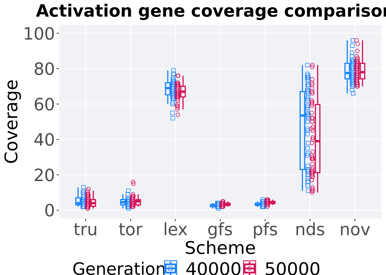
5.4.2.3 Stats

Summary statistics for the activation gene coverage at 40,000 and 50,000 generations.

slices = filter(cc_over_time_mvc, diagnostic == 'multipath_exploration' & (gen == 50000 | gen == 40000) & acron != 'ran')
slices$Generation <- factor(slices$gen, levels = c(50000,40000))
slices$acron = factor(slices$acron, levels = c('nov','lex', 'nds','tru','tor','gfs','pfs','ran'))
slices %>%
  group_by(acron, Generation) %>%
  dplyr::summarise(
    count = n(),
    na_cnt = sum(is.na(uni_str_pos)),
    min = min(uni_str_pos, na.rm = TRUE),
    median = median(uni_str_pos, na.rm = TRUE),
    mean = mean(uni_str_pos, na.rm = TRUE),
    max = max(uni_str_pos, na.rm = TRUE),
    IQR = IQR(uni_str_pos, na.rm = TRUE)
  )

## `summarise()` has grouped output by 'acron'. You can override using the
## `.groups` argument.

## # A tibble: 14 x 9
## # Groups:   acron [7]
##    acron Generation count na_cnt   min median  mean   max   IQR
##    <fct> <fct>      <int>  <int> <int>  <dbl> <dbl> <int> <dbl>
##  1 nov   50000         50      0    70   78   79.1     96  8.75
##  2 nov   40000         50      0    66   77.5 78.6     96  8.75
##  3 lex   50000         50      0    54   67   66.6     76  6   
##  4 lex   40000         50      0    52   69   68.3     79  6.75
##  5 nds   50000         50      0    10   39   40.4     82 38.5 
##  6 nds   40000         50      0    11   53.5 47.5     82 44   
##  7 tru   50000         50      0     1    4    4.8     12  3.75
##  8 tru   40000         50      0     2    4    4.78    13  4   
##  9 tor   50000         50      0     2    5    5.1     16  3   
## 10 tor   40000         50      0     1    4.5  4.38    11  3   
## 11 gfs   50000         50      0     2    3    3.14     5  1   
## 12 gfs   40000         50      0     1    3    2.72     4  1   
## 13 pfs   50000         50      0     2    4    4.34     6  1   
## 14 pfs   40000         50      0     2    3    3.28     6  1

Truncation selection comparisons.

wilcox.test(x = filter(slices, acron == 'tru' & Generation == 50000)$uni_str_pos,
            y = filter(slices, acron == 'tru' & Generation == 40000)$uni_str_pos,
            alternative = 't')

## 
##  Wilcoxon rank sum test with continuity correction
## 
## data:  filter(slices, acron == "tru" & Generation == 50000)$uni_str_pos and filter(slices, acron == "tru" & Generation == 40000)$uni_str_pos
## W = 1254.5, p-value = 0.9778
## alternative hypothesis: true location shift is not equal to 0

Tournament selection comparisons.

wilcox.test(x = filter(slices, acron == 'tor' & Generation == 50000)$uni_str_pos,
            y = filter(slices, acron == 'tor' & Generation == 40000)$uni_str_pos,
            alternative = 't')

## 
##  Wilcoxon rank sum test with continuity correction
## 
## data:  filter(slices, acron == "tor" & Generation == 50000)$uni_str_pos and filter(slices, acron == "tor" & Generation == 40000)$uni_str_pos
## W = 1396, p-value = 0.3094
## alternative hypothesis: true location shift is not equal to 0

Lexicase selection comparisons.

wilcox.test(x = filter(slices, acron == 'lex' & Generation == 50000)$uni_str_pos,
            y = filter(slices, acron == 'lex' & Generation == 40000)$uni_str_pos,
            alternative = 't')

## 
##  Wilcoxon rank sum test with continuity correction
## 
## data:  filter(slices, acron == "lex" & Generation == 50000)$uni_str_pos and filter(slices, acron == "lex" & Generation == 40000)$uni_str_pos
## W = 992.5, p-value = 0.07568
## alternative hypothesis: true location shift is not equal to 0

Genotypic fitness sharing comparisons.

wilcox.test(x = filter(slices, acron == 'gfs' & Generation == 50000)$uni_str_pos,
            y = filter(slices, acron == 'gfs' & Generation == 40000)$uni_str_pos,
            alternative = 't')

## 
##  Wilcoxon rank sum test with continuity correction
## 
## data:  filter(slices, acron == "gfs" & Generation == 50000)$uni_str_pos and filter(slices, acron == "gfs" & Generation == 40000)$uni_str_pos
## W = 1573, p-value = 0.01769
## alternative hypothesis: true location shift is not equal to 0

Phenotypic fitness sharing comparisons.

wilcox.test(x = filter(slices, acron == 'pfs' & Generation == 50000)$uni_str_pos,
            y = filter(slices, acron == 'pfs' & Generation == 40000)$uni_str_pos,
            alternative = 't')

## 
##  Wilcoxon rank sum test with continuity correction
## 
## data:  filter(slices, acron == "pfs" & Generation == 50000)$uni_str_pos and filter(slices, acron == "pfs" & Generation == 40000)$uni_str_pos
## W = 1914.5, p-value = 2.023e-06
## alternative hypothesis: true location shift is not equal to 0

Nondominated sorting comparisons.

wilcox.test(x = filter(slices, acron == 'nds' & Generation == 50000)$uni_str_pos,
            y = filter(slices, acron == 'nds' & Generation == 40000)$uni_str_pos,
            alternative = 't')

## 
##  Wilcoxon rank sum test with continuity correction
## 
## data:  filter(slices, acron == "nds" & Generation == 50000)$uni_str_pos and filter(slices, acron == "nds" & Generation == 40000)$uni_str_pos
## W = 1008, p-value = 0.09584
## alternative hypothesis: true location shift is not equal to 0

Novelty search comparisons.

wilcox.test(x = filter(slices, acron == 'nov' & Generation == 50000)$uni_str_pos,
            y = filter(slices, acron == 'nov' & Generation == 40000)$uni_str_pos,
            alternative = 't')

## 
##  Wilcoxon rank sum test with continuity correction
## 
## data:  filter(slices, acron == "nov" & Generation == 50000)$uni_str_pos and filter(slices, acron == "nov" & Generation == 40000)$uni_str_pos
## W = 1295.5, p-value = 0.756
## alternative hypothesis: true location shift is not equal to 0