Chapter 4 Contradictory objectives results

Here we present the results for the satisfactory trait corverage and activation gene coverage generated by each selection scheme replicate on the contradictory objectives diagnostic. Note both of these values are gathered at the population-level. Activation gene coverage refers to the count of unique activation genes in a given population; this gives us a range of integers between 0 and 100. Satisfactory trait coverage refers to the count of unique satisfied traits in a given population; this gives us a range of integers between 0 and 100.

4.1 Analysis dependencies

library(ggplot2)
library(cowplot)
library(dplyr)
library(PupillometryR)
library(sdamr)

4.2 Satisfactory trait coverage

Satisfactory trait coverage analysis.

4.2.1 Coverage over time

Satisfactory trait coverage over time.

# data for lines and shading on plots
lines = filter(cc_over_time, diagnostic == 'contradictory_objectives') %>%
  group_by(`Selection\nScheme`, gen) %>%
  dplyr::summarise(
    min = min(pop_uni_obj),
    mean = mean(pop_uni_obj),
    max = max(pop_uni_obj)
  )

## `summarise()` has grouped output by 'Selection Scheme'. You can override using
## the `.groups` argument.

ggplot(lines, aes(x=gen, y=mean, group = `Selection\nScheme`, fill =`Selection\nScheme`, color = `Selection\nScheme`, shape = `Selection\nScheme`)) +
  geom_ribbon(aes(ymin = min, ymax = max), alpha = 0.1) +
  geom_line(size = 0.5) +
  geom_point(data = filter(lines, gen %% 2000 == 0 & gen != 0), size = 1.5, stroke = 2.0, alpha = 1.0) +
  scale_y_continuous(
    name="Coverage",
    limits=c(0, 100),
    breaks=seq(0,100, 20),
    labels=c("0", "20", "40", "60", "80", "100")
  ) +
  scale_x_continuous(
    name="Generations",
    limits=c(0, 50000),
    breaks=c(0, 10000, 20000, 30000, 40000, 50000),
    labels=c("0e+4", "1e+4", "2e+4", "3e+4", "4e+4", "5e+4")
  ) +
  scale_shape_manual(values=SHAPE)+
  scale_colour_manual(values = cb_palette) +
  scale_fill_manual(values = cb_palette) +
  ggtitle('Satisfactory trait coverage over time')+
  p_theme + theme(legend.title=element_blank(),legend.text=element_text(size=11)) +
  guides(
    shape=guide_legend(ncol=2, title.position = "bottom"),
    color=guide_legend(ncol=2, title.position = "bottom"),
    fill=guide_legend(ncol=2, title.position = "bottom")
  )

4.2.2 Best coverage throughout

Best satisfactory trait coverage throughout 50,000 generations.

### best satisfactory trait coverage throughout
filter(cc_best, col == 'pop_uni_obj' & diagnostic == 'contradictory_objectives') %>%
  ggplot(., aes(x = acron, y = val, color = acron, fill = acron, shape = acron)) +
  geom_flat_violin(position = position_nudge(x = .2, y = 0), scale = 'width', alpha = 0.2) +
  geom_point(position = position_jitter(width = .1), size = 1.5, alpha = 1.0) +
  geom_boxplot(color = 'black', width = .2, outlier.shape = NA, alpha = 0.0) +
  scale_y_continuous(
    name="Coverage",
    limits=c(0, 100),
    breaks=seq(0,100, 20),
    labels=c("0", "20", "40", "60", "80", "100")
  ) +
  scale_x_discrete(
    name="Scheme"
  )+
  scale_shape_manual(values=SHAPE)+
  scale_colour_manual(values = cb_palette, ) +
  scale_fill_manual(values = cb_palette) +
  ggtitle('Best satisfactory trait coverage')+
  p_theme + theme(legend.title=element_blank()) +
  guides(
    shape=guide_legend(nrow=2, title.position = "bottom"),
    color=guide_legend(nrow=2, title.position = "bottom"),
    fill=guide_legend(nrow=2, title.position = "bottom")
  )

## Warning: Removed 50 rows containing missing values (`geom_point()`).

4.2.2.1 Stats

Summary statistics for the best satisfactory trait coverage.

### best
coverage = filter(cc_best, col == 'pop_uni_obj' & diagnostic == 'contradictory_objectives')
coverage$acron = factor(coverage$acron, levels = c('nds', 'lex', 'pfs', 'gfs', 'tor', 'tru', 'nov', 'ran'))
coverage %>%
  group_by(acron) %>%
  dplyr::summarise(
    count = n(),
    na_cnt = sum(is.na(val)),
    min = min(val, na.rm = TRUE),
    median = median(val, na.rm = TRUE),
    mean = mean(val, na.rm = TRUE),
    max = max(val, na.rm = TRUE),
    IQR = IQR(val, na.rm = TRUE)
  )

## # A tibble: 8 x 8
##   acron count na_cnt   min median  mean   max   IQR
##   <fct> <int>  <int> <dbl>  <dbl> <dbl> <dbl> <dbl>
## 1 nds      50      0    85     91 91.8    100     5
## 2 lex      50      0    45     48 48.2     51     2
## 3 pfs      50      0     3      4  3.84     6     1
## 4 gfs      50      0     1      1  1        1     0
## 5 tor      50      0     1      1  1        1     0
## 6 tru      50      0     1      1  1        1     0
## 7 nov      50      0     0      0  0        0     0
## 8 ran      50      0     0      0  0        0     0

Kruskal–Wallis test provides evidence of difference among satisfactory trait coverage.

kruskal.test(val ~ acron, data = coverage)

## 
##  Kruskal-Wallis rank sum test
## 
## data:  val by acron
## Kruskal-Wallis chi-squared = 396.67, df = 7, p-value < 2.2e-16

Results for post-hoc Wilcoxon rank-sum test with a Bonferroni correction on satisfactory trait coverage.

pairwise.wilcox.test(x = coverage$val, g = coverage$acron, p.adjust.method = "bonferroni",
                     paired = FALSE, conf.int = FALSE, alternative = 'l')

## 
##  Pairwise comparisons using Wilcoxon rank sum test with continuity correction 
## 
## data:  coverage$val and coverage$acron 
## 
##     nds    lex    pfs    gfs    tor    tru    nov
## lex <2e-16 -      -      -      -      -      -  
## pfs <2e-16 <2e-16 -      -      -      -      -  
## gfs <2e-16 <2e-16 <2e-16 -      -      -      -  
## tor <2e-16 <2e-16 <2e-16 1      -      -      -  
## tru <2e-16 <2e-16 <2e-16 1      1      -      -  
## nov <2e-16 <2e-16 <2e-16 <2e-16 <2e-16 <2e-16 -  
## ran <2e-16 <2e-16 <2e-16 <2e-16 <2e-16 <2e-16 1  
## 
## P value adjustment method: bonferroni

4.2.3 End of 50,000 generations

Satisfactory trait coverage in the population at the end of 50,000 generations.

### end of run
filter(cc_over_time, diagnostic == 'contradictory_objectives' & gen == 50000) %>%
  ggplot(., aes(x = acron, y = pop_uni_obj, color = acron, fill = acron, shape = acron)) +
  geom_flat_violin(position = position_nudge(x = .2, y = 0), scale = 'width', alpha = 0.2) +
  geom_point(position = position_jitter(width = .1), size = 1.5, alpha = 1.0) +
  geom_boxplot(color = 'black', width = .2, outlier.shape = NA, alpha = 0.0) +
  scale_y_continuous(
    name="Coverage",
    limits=c(0, 100),
    breaks=seq(0,100, 20),
    labels=c("0", "20", "40", "60", "80", "100")
  ) +
  scale_x_discrete(
    name="Scheme"
  )+
  scale_shape_manual(values=SHAPE)+
  scale_colour_manual(values = cb_palette, ) +
  scale_fill_manual(values = cb_palette) +
  ggtitle('Final satisfactory trait coverage')+
  p_theme + theme(legend.title=element_blank()) +
  guides(
    shape=guide_legend(nrow=2, title.position = "bottom"),
    color=guide_legend(nrow=2, title.position = "bottom"),
    fill=guide_legend(nrow=2, title.position = "bottom")
  )

## Warning: Removed 52 rows containing missing values (`geom_point()`).

4.2.3.1 Stats

Summary statistics for satisfactory trait coverage in the population at the end of 50,000 generations.

### end of run
coverage = filter(cc_over_time, diagnostic == 'contradictory_objectives' & gen == 50000)
coverage$acron = factor(coverage$acron, levels = c('nds', 'lex', 'pfs', 'gfs', 'tor', 'tru', 'nov', 'ran'))
coverage %>%
  group_by(acron) %>%
  dplyr::summarise(
    count = n(),
    na_cnt = sum(is.na(pop_uni_obj)),
    min = min(pop_uni_obj, na.rm = TRUE),
    median = median(pop_uni_obj, na.rm = TRUE),
    mean = mean(pop_uni_obj, na.rm = TRUE),
    max = max(pop_uni_obj, na.rm = TRUE),
    IQR = IQR(pop_uni_obj, na.rm = TRUE)
  )

## # A tibble: 8 x 8
##   acron count na_cnt   min median  mean   max   IQR
##   <fct> <int>  <int> <int>  <dbl> <dbl> <int> <dbl>
## 1 nds      50      0    82     86 86.4     92     3
## 2 lex      50      0    36     39 38.6     40     1
## 3 pfs      50      0     3      4  3.82     6     1
## 4 gfs      50      0     1      1  1        1     0
## 5 tor      50      0     1      1  1        1     0
## 6 tru      50      0     1      1  1        1     0
## 7 nov      50      0     0      0  0        0     0
## 8 ran      50      0     0      0  0        0     0

Kruskal–Wallis test provides evidence of difference among satisfactory trait coverage in the population at the end of 50,000 generations.

kruskal.test(pop_uni_obj ~ acron, data = coverage)

## 
##  Kruskal-Wallis rank sum test
## 
## data:  pop_uni_obj by acron
## Kruskal-Wallis chi-squared = 396.7, df = 7, p-value < 2.2e-16

Results for post-hoc Wilcoxon rank-sum test with a Bonferroni correction on satisfactory trait coverage in the population at the end of 50,000 generations.

pairwise.wilcox.test(x = coverage$pop_uni_obj, g = coverage$acron, p.adjust.method = "bonferroni",
                     paired = FALSE, conf.int = FALSE, alternative = 'l')

## 
##  Pairwise comparisons using Wilcoxon rank sum test with continuity correction 
## 
## data:  coverage$pop_uni_obj and coverage$acron 
## 
##     nds    lex    pfs    gfs    tor    tru    nov
## lex <2e-16 -      -      -      -      -      -  
## pfs <2e-16 <2e-16 -      -      -      -      -  
## gfs <2e-16 <2e-16 <2e-16 -      -      -      -  
## tor <2e-16 <2e-16 <2e-16 1      -      -      -  
## tru <2e-16 <2e-16 <2e-16 1      1      -      -  
## nov <2e-16 <2e-16 <2e-16 <2e-16 <2e-16 <2e-16 -  
## ran <2e-16 <2e-16 <2e-16 <2e-16 <2e-16 <2e-16 1  
## 
## P value adjustment method: bonferroni

4.3 Activation gene coverage

Activation gene coverage analysis.

4.3.1 Over time coverage

Activation gene coverage over time.

# data for lines and shading on plots
lines = filter(cc_over_time, diagnostic == 'contradictory_objectives') %>%
  group_by(`Selection\nScheme`, gen) %>%
  dplyr::summarise(
    min = min(uni_str_pos),
    mean = mean(uni_str_pos),
    max = max(uni_str_pos)
  )

## `summarise()` has grouped output by 'Selection Scheme'. You can override using
## the `.groups` argument.

ggplot(lines, aes(x=gen, y=mean, group = `Selection\nScheme`, fill =`Selection\nScheme`, color = `Selection\nScheme`, shape = `Selection\nScheme`)) +
  geom_ribbon(aes(ymin = min, ymax = max), alpha = 0.1) +
  geom_line(size = 0.5) +
  geom_point(data = filter(lines, gen %% 2000 == 0 & gen != 0), size = 1.5, stroke = 2.0, alpha = 1.0) +
  scale_y_continuous(
    name="Coverage",
    limits=c(0, 100),
    breaks=seq(0,100, 20),
    labels=c("0", "20", "40", "60", "80", "100")
  ) +
  scale_x_continuous(
    name="Generations",
    limits=c(0, 50000),
    breaks=c(0, 10000, 20000, 30000, 40000, 50000),
    labels=c("0e+4", "1e+4", "2e+4", "3e+4", "4e+4", "5e+4")
  ) +
  scale_shape_manual(values=SHAPE)+
  scale_colour_manual(values = cb_palette) +
  scale_fill_manual(values = cb_palette) +
  ggtitle('Activation gene coverage over time')+
  p_theme + theme(legend.title=element_blank(),legend.text=element_text(size=11)) +
  guides(
    shape=guide_legend(ncol=2, title.position = "bottom"),
    color=guide_legend(ncol=2, title.position = "bottom"),
    fill=guide_legend(ncol=2, title.position = "bottom")
  )

4.3.2 End of 50,000 generations

Activation gene coverage in the population at the end of 50,000 generations.

# end of run
filter(cc_over_time, diagnostic == 'contradictory_objectives' & gen == 50000) %>%
  ggplot(., aes(x = acron, y = uni_str_pos, color = acron, fill = acron, shape = acron)) +
  geom_flat_violin(position = position_nudge(x = .2, y = 0), scale = 'width', alpha = 0.2) +
  geom_point(position = position_jitter(width = .1), size = 1.5, alpha = 1.0) +
  geom_boxplot(color = 'black', width = .2, outlier.shape = NA, alpha = 0.0) +
  scale_y_continuous(
    name="Coverage",
    limits=c(0, 100),
    breaks=seq(0,100, 20),
    labels=c("0", "20", "40", "60", "80", "100")
  ) +
  scale_x_discrete(
    name="Scheme"
  )+
  scale_shape_manual(values=SHAPE)+
  scale_colour_manual(values = cb_palette, ) +
  scale_fill_manual(values = cb_palette) +
  ggtitle('Final activation gene coverage')+
  p_theme + theme(legend.title=element_blank()) +
  guides(
    shape=guide_legend(nrow=2, title.position = "bottom"),
    color=guide_legend(nrow=2, title.position = "bottom"),
    fill=guide_legend(nrow=2, title.position = "bottom")
  )

## Warning: Removed 17 rows containing missing values (`geom_point()`).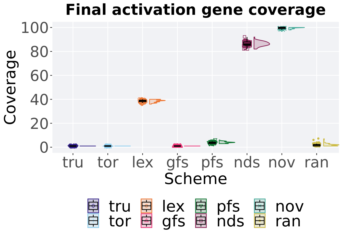

4.3.2.1 Stats

Summary statistics for activation gene coverage.

# end of run
coverage = filter(cc_over_time, diagnostic == 'contradictory_objectives' & gen == 50000)
coverage$acron = factor(coverage$acron, levels = c('nov', 'nds', 'lex', 'pfs', 'ran', 'gfs', 'tor', 'tru'))
coverage %>%
  group_by(acron) %>%
  dplyr::summarise(
    count = n(),
    na_cnt = sum(is.na(uni_str_pos)),
    min = min(uni_str_pos, na.rm = TRUE),
    median = median(uni_str_pos, na.rm = TRUE),
    mean = mean(uni_str_pos, na.rm = TRUE),
    max = max(uni_str_pos, na.rm = TRUE),
    IQR = IQR(uni_str_pos, na.rm = TRUE)
  )

## # A tibble: 8 x 8
##   acron count na_cnt   min median  mean   max   IQR
##   <fct> <int>  <int> <int>  <dbl> <dbl> <int> <dbl>
## 1 nov      50      0    98    100 99.6    100     1
## 2 nds      50      0    82     86 86.4     92     3
## 3 lex      50      0    36     39 38.6     40     1
## 4 pfs      50      0     3      4  3.98     6     1
## 5 ran      50      0     1      2  2.06     7     1
## 6 gfs      50      0     1      1  1        1     0
## 7 tor      50      0     1      1  1        1     0
## 8 tru      50      0     1      1  1        1     0

Kruskal–Wallis test provides evidence of difference among activation gene coverage.

kruskal.test(uni_str_pos ~ acron, data = coverage)

## 
##  Kruskal-Wallis rank sum test
## 
## data:  uni_str_pos by acron
## Kruskal-Wallis chi-squared = 384.23, df = 7, p-value < 2.2e-16

Results for post-hoc Wilcoxon rank-sum test with a Bonferroni correction on activation gene coverage.

pairwise.wilcox.test(x = coverage$uni_str_pos, g = coverage$acron, p.adjust.method = "bonferroni",
                     paired = FALSE, conf.int = FALSE, alternative = 'l')

## 
##  Pairwise comparisons using Wilcoxon rank sum test with continuity correction 
## 
## data:  coverage$uni_str_pos and coverage$acron 
## 
##     nov     nds     lex     pfs     ran     gfs tor
## nds < 2e-16 -       -       -       -       -   -  
## lex < 2e-16 < 2e-16 -       -       -       -   -  
## pfs < 2e-16 < 2e-16 < 2e-16 -       -       -   -  
## ran < 2e-16 < 2e-16 < 2e-16 2.9e-12 -       -   -  
## gfs < 2e-16 < 2e-16 < 2e-16 < 2e-16 3.0e-10 -   -  
## tor < 2e-16 < 2e-16 < 2e-16 < 2e-16 3.0e-10 1   -  
## tru < 2e-16 < 2e-16 < 2e-16 < 2e-16 3.0e-10 1   1  
## 
## P value adjustment method: bonferroni

4.4 Nondominated sorting split

Here analyze the satisfactory trait coverage and activation gene coverage results for nondominated sorting, nondominated front ranking (no fitness sharing between fronts), and phenotypic fitness sharing.

4.4.1 Coverage over time

Satisfactory trait coverage over time.

lines = filter(nss, diagnostic == 'contradictory_objectives') %>%
  group_by(`Selection\nScheme`, gen) %>%
  dplyr::summarise(
    min = min(pop_uni_obj),
    mean = mean(pop_uni_obj),
    max = max(pop_uni_obj)
  )

## `summarise()` has grouped output by 'Selection Scheme'. You can override using
## the `.groups` argument.

ggplot(lines, aes(x=gen, y=mean, group = `Selection\nScheme`, fill =`Selection\nScheme`, color = `Selection\nScheme`, shape = `Selection\nScheme`)) +
  geom_ribbon(aes(ymin = min, ymax = max), alpha = 0.1) +
  geom_line(size = 0.5) +
  geom_point(data = filter(lines, gen %% 2000 == 0 & gen != 0), size = 1.5, stroke = 2.0, alpha = 1.0) +
  scale_y_continuous(
    name="Coverage",
    limits=c(0, 100),
    breaks=seq(0,100, 20),
    labels=c("0", "20", "40", "60", "80", "100")
  ) +
  scale_x_continuous(
    name="Generations",
    limits=c(0, 50000),
    breaks=c(0, 10000, 20000, 30000, 40000, 50000),
    labels=c("0e+4", "1e+4", "2e+4", "3e+4", "4e+4", "5e+4")
  ) +
  scale_shape_manual(values=SHAPE)+
  scale_colour_manual(values = cb_palette) +
  scale_fill_manual(values = cb_palette) +
  ggtitle('Satisfactory trait coverage over time')+
  p_theme + theme(legend.title=element_blank(),legend.text=element_text(size=11)) +
  guides(
    shape=guide_legend(ncol=1, title.position = "bottom"),
    color=guide_legend(ncol=1, title.position = "bottom"),
    fill=guide_legend(ncol=1, title.position = "bottom")
  )

4.4.2 Best coverage throughout

Best satisfactory trait coverage.

### best satisfactory trait coverage throughout
coverage %>%
  ggplot(., aes(x = acron, y = val, color = acron, fill = acron, shape = acron)) +
  geom_flat_violin(position = position_nudge(x = .2, y = 0), scale = 'width', alpha = 0.2) +
  geom_point(position = position_jitter(width = .1), size = 1.5, alpha = 1.0) +
  geom_boxplot(color = 'black', width = .2, outlier.shape = NA, alpha = 0.0) +
  scale_y_continuous(
    name="Coverage",
    limits=c(0, 100),
    breaks=seq(0,100, 20),
    labels=c("0", "20", "40", "60", "80", "100")
  ) +
  scale_x_discrete(
    name="Scheme"
  )+
  scale_shape_manual(values=SHAPE)+
  scale_colour_manual(values = cb_palette, ) +
  scale_fill_manual(values = cb_palette) +
  ggtitle('Best satisfactory trait coverage')+
  p_theme + theme(legend.title=element_blank()) +
  guides(
    shape=guide_legend(nrow=1, title.position = "bottom"),
    color=guide_legend(nrow=1, title.position = "bottom"),
    fill=guide_legend(nrow=1, title.position = "bottom")
  )

## Warning: Removed 2 rows containing missing values (`geom_point()`).

4.4.2.1 Stats

Summary statistics for the best satisfactory trait coverage.

# summary
coverage$acron = factor(coverage$acron, levels = c('nds', 'pfs', 'nfr'))
coverage %>%
  group_by(acron) %>%
  dplyr::summarise(
    count = n(),
    na_cnt = sum(is.na(val)),
    min = min(val, na.rm = TRUE),
    median = median(val, na.rm = TRUE),
    mean = mean(val, na.rm = TRUE),
    max = max(val, na.rm = TRUE),
    IQR = IQR(val, na.rm = TRUE)
  )

## # A tibble: 3 x 8
##   acron count na_cnt   min median  mean   max   IQR
##   <fct> <int>  <int> <dbl>  <dbl> <dbl> <dbl> <dbl>
## 1 nds      50      0    85     91  91.8   100   5  
## 2 pfs      50      0     1      1   1       1   0  
## 3 nfr      50      0    28     44  42.8    54   8.5

Kruskal–Wallis test provides evidence of difference among best satisfactory trait coverage.

kruskal.test(val ~ acron,data = coverage)

## 
##  Kruskal-Wallis rank sum test
## 
## data:  val by acron
## Kruskal-Wallis chi-squared = 137.61, df = 2, p-value < 2.2e-16

Results for post-hoc Wilcoxon rank-sum test with a Bonferroni correction on best satisfactory trait coverage.

pairwise.wilcox.test(x = coverage$val, g = coverage$acron, p.adjust.method = "bonferroni",
                     paired = FALSE, conf.int = FALSE, alternative = 'l')

## 
##  Pairwise comparisons using Wilcoxon rank sum test with continuity correction 
## 
## data:  coverage$val and coverage$acron 
## 
##     nds    pfs
## pfs <2e-16 -  
## nfr <2e-16 1  
## 
## P value adjustment method: bonferroni

4.4.3 End of 50,000 generations

Satisfactory trait coverage in the population at the end of 50,000 generations.

coverage %>%
  ggplot(., aes(x = acron, y = pop_uni_obj, color = acron, fill = acron, shape = acron)) +
  geom_flat_violin(position = position_nudge(x = .2, y = 0), scale = 'width', alpha = 0.2) +
  geom_point(position = position_jitter(width = .1), size = 1.5, alpha = 1.0) +
  geom_boxplot(color = 'black', width = .2, outlier.shape = NA, alpha = 0.0) +
  scale_y_continuous(
    name="Coverage",
    limits=c(0, 100),
    breaks=seq(0,100, 20),
    labels=c("0", "20", "40", "60", "80", "100")
  ) +
  scale_x_discrete(
    name="Scheme"
  )+
  scale_shape_manual(values=SHAPE)+
  scale_colour_manual(values = cb_palette, ) +
  scale_fill_manual(values = cb_palette) +
  ggtitle('Final satisfactory trait coverage')+
  p_theme + theme(legend.title=element_blank()) +
  guides(
    shape=guide_legend(nrow=1, title.position = "bottom"),
    color=guide_legend(nrow=1, title.position = "bottom"),
    fill=guide_legend(nrow=1, title.position = "bottom")
  )

4.4.3.1 Stats

Summary statistics for satisfactory trait coverage in the population at the end of 50,000 generations.

coverage$acron = factor(coverage$acron, levels = c('nds', 'pfs', 'nfr'))
coverage %>%
  group_by(acron) %>%
  dplyr::summarise(
    count = n(),
    na_cnt = sum(is.na(pop_uni_obj)),
    min = min(pop_uni_obj, na.rm = TRUE),
    median = median(pop_uni_obj, na.rm = TRUE),
    mean = mean(pop_uni_obj, na.rm = TRUE),
    max = max(pop_uni_obj, na.rm = TRUE),
    IQR = IQR(pop_uni_obj, na.rm = TRUE)
  )

## # A tibble: 3 x 8
##   acron count na_cnt   min median  mean   max   IQR
##   <fct> <int>  <int> <int>  <dbl> <dbl> <int> <dbl>
## 1 nds      50      0    82     86 86.4     92     3
## 2 pfs      50      0     3      4  3.82     6     1
## 3 nfr      50      0     1      1  1.28     2     1

Kruskal–Wallis test provides evidence of difference among satisfactory trait coverage in the population at the end of 50,000 generations.

kruskal.test(pop_uni_obj ~ acron,data = coverage)

## 
##  Kruskal-Wallis rank sum test
## 
## data:  pop_uni_obj by acron
## Kruskal-Wallis chi-squared = 135.36, df = 2, p-value < 2.2e-16

Results for post-hoc Wilcoxon rank-sum test with a Bonferroni correction on satisfactory trait coverage in the population at the end of 50,000 generations.

pairwise.wilcox.test(x = coverage$pop_uni_obj, g = coverage$acron, p.adjust.method = "bonferroni",
                     paired = FALSE, conf.int = FALSE, alternative = 'l')

## 
##  Pairwise comparisons using Wilcoxon rank sum test with continuity correction 
## 
## data:  coverage$pop_uni_obj and coverage$acron 
## 
##     nds    pfs   
## pfs <2e-16 -     
## nfr <2e-16 <2e-16
## 
## P value adjustment method: bonferroni

4.5 Multi-valley crossing results

4.5.1 Satisfactory trait coverage

Satisfactory trait coverage analysis.

4.5.1.1 Coverage over time

Satisfactory trait coverage over time.

# data for lines and shading on plots
lines = filter(cc_over_time_mvc, diagnostic == 'contradictory_objectives') %>%
  group_by(`Selection\nScheme`, gen) %>%
  dplyr::summarise(
    min = min(pop_uni_obj),
    mean = mean(pop_uni_obj),
    max = max(pop_uni_obj)
  )

## `summarise()` has grouped output by 'Selection Scheme'. You can override using
## the `.groups` argument.

ggplot(lines, aes(x=gen, y=mean, group = `Selection\nScheme`, fill =`Selection\nScheme`, color = `Selection\nScheme`, shape = `Selection\nScheme`)) +
  geom_ribbon(aes(ymin = min, ymax = max), alpha = 0.1) +
  geom_line(size = 0.5) +
  geom_point(data = filter(lines, gen %% 2000 == 0 & gen != 0), size = 1.5, stroke = 2.0, alpha = 1.0) +
  scale_y_continuous(
    name="Coverage",
    limits=c(0, 5),
    breaks=seq(0,5, 1)
  ) +
  scale_x_continuous(
    name="Generations",
    limits=c(0, 50000),
    breaks=c(0, 10000, 20000, 30000, 40000, 50000),
    labels=c("0e+4", "1e+4", "2e+4", "3e+4", "4e+4", "5e+4")
  ) +
  scale_shape_manual(values=SHAPE)+
  scale_colour_manual(values = cb_palette) +
  scale_fill_manual(values = cb_palette) +
  ggtitle('Satisfactory trait coverage over time')+
  p_theme + theme(legend.title=element_blank(),legend.text=element_text(size=11)) +
  guides(
    shape=guide_legend(ncol=2, title.position = "bottom"),
    color=guide_legend(ncol=2, title.position = "bottom"),
    fill=guide_legend(ncol=2, title.position = "bottom")
  )

4.5.1.2 Best coverage throughout

Best satisfactory trait coverage throughout 50,000 generations.

### best satisfactory trait coverage throughout
filter(cc_best_mvc, col == 'pop_uni_obj' & diagnostic == 'contradictory_objectives') %>%
  ggplot(., aes(x = acron, y = val, color = acron, fill = acron, shape = acron)) +
  geom_flat_violin(position = position_nudge(x = .2, y = 0), scale = 'width', alpha = 0.2) +
  geom_point(position = position_jitter(width = .1), size = 1.5, alpha = 1.0) +
  geom_boxplot(color = 'black', width = .2, outlier.shape = NA, alpha = 0.0) +
  guides(fill = "none",color = 'none', shape = 'none') +
  scale_y_continuous(
    name="Coverage",
    limits=c(0, 5)
  ) +
  scale_x_discrete(
    name="Scheme"
  )+
  scale_shape_manual(values=SHAPE)+
  scale_colour_manual(values = cb_palette, ) +
  scale_fill_manual(values = cb_palette) +
  ggtitle('Best satisfactory trait coverage')+
  p_theme + theme(legend.title=element_blank()) +
  guides(
    shape=guide_legend(nrow=2, title.position = "bottom"),
    color=guide_legend(nrow=2, title.position = "bottom"),
    fill=guide_legend(nrow=2, title.position = "bottom")
  )

## Warning: Removed 178 rows containing missing values (`geom_point()`).

4.5.1.2.1 Stats

Summary statistics for the best satisfactory trait coverage.

### best
coverage = filter(cc_best_mvc, col == 'pop_uni_obj' & diagnostic == 'contradictory_objectives')
coverage$acron = factor(coverage$acron, levels = c('pfs','nds', 'lex',  'gfs', 'tor', 'tru', 'nov', 'ran'))
coverage %>%
  group_by(acron) %>%
  dplyr::summarise(
    count = n(),
    na_cnt = sum(is.na(val)),
    min = min(val, na.rm = TRUE),
    median = median(val, na.rm = TRUE),
    mean = mean(val, na.rm = TRUE),
    max = max(val, na.rm = TRUE),
    IQR = IQR(val, na.rm = TRUE)
  )

## # A tibble: 8 x 8
##   acron count na_cnt   min median  mean   max   IQR
##   <fct> <int>  <int> <dbl>  <dbl> <dbl> <dbl> <dbl>
## 1 pfs      50      0     2      3  3.42     5     1
## 2 nds      50      0     0      0  0        0     0
## 3 lex      50      0     0      0  0        0     0
## 4 gfs      50      0     0      0  0        0     0
## 5 tor      50      0     0      0  0        0     0
## 6 tru      50      0     0      0  0        0     0
## 7 nov      50      0     0      0  0        0     0
## 8 ran      50      0     0      0  0        0     0

Kruskal–Wallis test provides evidence of difference among satisfactory trait coverage.

kruskal.test(val ~ acron, data = coverage)

## 
##  Kruskal-Wallis rank sum test
## 
## data:  val by acron
## Kruskal-Wallis chi-squared = 396.91, df = 7, p-value < 2.2e-16

Results for post-hoc Wilcoxon rank-sum test with a Bonferroni correction on satisfactory trait coverage.

pairwise.wilcox.test(x = coverage$val, g = coverage$acron, p.adjust.method = "bonferroni",
                     paired = FALSE, conf.int = FALSE, alternative = 'l')

## 
##  Pairwise comparisons using Wilcoxon rank sum test with continuity correction 
## 
## data:  coverage$val and coverage$acron 
## 
##     pfs    nds lex gfs tor tru nov
## nds <2e-16 -   -   -   -   -   -  
## lex <2e-16 1   -   -   -   -   -  
## gfs <2e-16 1   1   -   -   -   -  
## tor <2e-16 1   1   1   -   -   -  
## tru <2e-16 1   1   1   1   -   -  
## nov <2e-16 1   1   1   1   1   -  
## ran <2e-16 1   1   1   1   1   1  
## 
## P value adjustment method: bonferroni

4.5.1.3 Coverage comparison

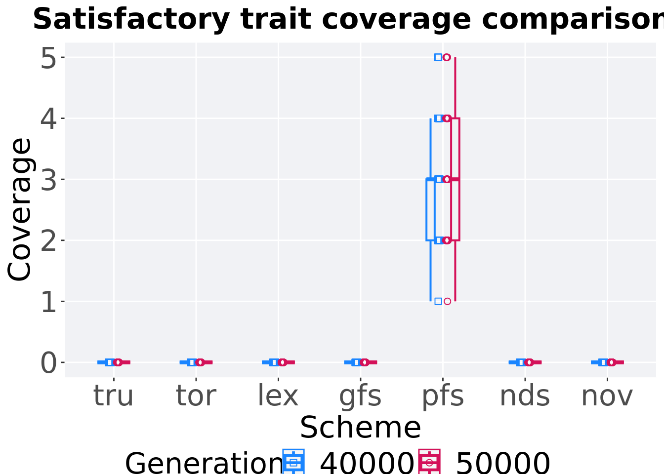
Best performances in the population at 40,000 and 50,000 generations.

## Warning: The following aesthetics were dropped during statistical transformation:
## colour, shape
## i This can happen when ggplot fails to infer the correct grouping structure in
##   the data.
## i Did you forget to specify a `group` aesthetic or to convert a numerical
##   variable into a factor?
## The following aesthetics were dropped during statistical transformation:
## colour, shape
## i This can happen when ggplot fails to infer the correct grouping structure in
##   the data.
## i Did you forget to specify a `group` aesthetic or to convert a numerical
##   variable into a factor?

end = filter(cc_over_time_mvc, diagnostic == 'contradictory_objectives' & gen == 50000 & acron != 'ran')
end$Generation <- factor(end$gen)

mid = filter(cc_over_time_mvc, diagnostic == 'contradictory_objectives' & gen == 40000 & acron != 'ran')
mid$Generation <- factor(mid$gen)

mvc_p = ggplot(mid, aes(x = acron, y=pop_uni_obj, group = acron, shape = Generation)) +
  geom_point(col = mvc_col[1] , position = position_jitternudge(jitter.width = .03, nudge.x = -0.05), size = 2, alpha = 1.0) +
  geom_boxplot(position = position_nudge(x = -.15, y = 0), lwd = 0.7, col = mvc_col[1], fill = mvc_col[1], width = .1, outlier.shape = NA, alpha = 0.0) +

  geom_point(data = end, aes(x = acron, y=pop_uni_obj), col = mvc_col[2], position = position_jitternudge(jitter.width = .03, nudge.x = 0.05), size = 2, alpha = 1.0) +
  geom_boxplot(data = end, aes(x = acron, y=pop_uni_obj), position = position_nudge(x = .15, y = 0), lwd = 0.7, col = mvc_col[2], fill = mvc_col[2], width = .1, outlier.shape = NA, alpha = 0.0) +

  scale_y_continuous(
    name="Coverage",
    limits=c(0, 5)
  ) +
  scale_x_discrete(
    name="Scheme"
  )+
  scale_shape_manual(values=c(0,1))+
  scale_colour_manual(values = c(mvc_col[1],mvc_col[2])) +
  p_theme

plot_grid(
  mvc_p +
    ggtitle("Satisfactory trait coverage comparisons") +
    theme(legend.position="none"),
  legend,
  nrow=2,
  rel_heights = c(1,.05),
  label_size = TSIZE
)

4.5.1.3.1 Stats

Summary statistics for the activation gene coverage at 40,000 and 50,000 generations.

slices = filter(cc_over_time_mvc, diagnostic == 'contradictory_objectives' & (gen == 50000 | gen == 40000) & acron != 'ran')
slices$Generation <- factor(slices$gen, levels = c(50000,40000))
slices$acron = factor(slices$acron, levels = c('pfs','nds', 'lex',  'gfs', 'tor', 'tru', 'nov', 'ran'))
slices %>%
  group_by(acron, Generation) %>%
  dplyr::summarise(
    count = n(),
    na_cnt = sum(is.na(pop_uni_obj)),
    min = min(pop_uni_obj, na.rm = TRUE),
    median = median(pop_uni_obj, na.rm = TRUE),
    mean = mean(pop_uni_obj, na.rm = TRUE),
    max = max(pop_uni_obj, na.rm = TRUE),
    IQR = IQR(pop_uni_obj, na.rm = TRUE)
  )

## `summarise()` has grouped output by 'acron'. You can override using the
## `.groups` argument.

## # A tibble: 14 x 9
## # Groups:   acron [7]
##    acron Generation count na_cnt   min median  mean   max   IQR
##    <fct> <fct>      <int>  <int> <int>  <dbl> <dbl> <int> <dbl>
##  1 pfs   50000         50      0     1      3  3.14     5     2
##  2 pfs   40000         50      0     1      3  2.9      5     1
##  3 nds   50000         50      0     0      0  0        0     0
##  4 nds   40000         50      0     0      0  0        0     0
##  5 lex   50000         50      0     0      0  0        0     0
##  6 lex   40000         50      0     0      0  0        0     0
##  7 gfs   50000         50      0     0      0  0        0     0
##  8 gfs   40000         50      0     0      0  0        0     0
##  9 tor   50000         50      0     0      0  0        0     0
## 10 tor   40000         50      0     0      0  0        0     0
## 11 tru   50000         50      0     0      0  0        0     0
## 12 tru   40000         50      0     0      0  0        0     0
## 13 nov   50000         50      0     0      0  0        0     0
## 14 nov   40000         50      0     0      0  0        0     0

Truncation selection comparisons.

wilcox.test(x = filter(slices, acron == 'tru' & Generation == 50000)$pop_uni_obj,
            y = filter(slices, acron == 'tru' & Generation == 40000)$pop_uni_obj,
            alternative = 't')

## 
##  Wilcoxon rank sum test with continuity correction
## 
## data:  filter(slices, acron == "tru" & Generation == 50000)$pop_uni_obj and filter(slices, acron == "tru" & Generation == 40000)$pop_uni_obj
## W = 1250, p-value = NA
## alternative hypothesis: true location shift is not equal to 0

Tournament selection comparisons.

wilcox.test(x = filter(slices, acron == 'tor' & Generation == 50000)$pop_uni_obj,
            y = filter(slices, acron == 'tor' & Generation == 40000)$pop_uni_obj,
            alternative = 't')

## 
##  Wilcoxon rank sum test with continuity correction
## 
## data:  filter(slices, acron == "tor" & Generation == 50000)$pop_uni_obj and filter(slices, acron == "tor" & Generation == 40000)$pop_uni_obj
## W = 1250, p-value = NA
## alternative hypothesis: true location shift is not equal to 0

Lexicase selection comparisons.

wilcox.test(x = filter(slices, acron == 'lex' & Generation == 50000)$pop_uni_obj,
            y = filter(slices, acron == 'lex' & Generation == 40000)$pop_uni_obj,
            alternative = 't')

## 
##  Wilcoxon rank sum test with continuity correction
## 
## data:  filter(slices, acron == "lex" & Generation == 50000)$pop_uni_obj and filter(slices, acron == "lex" & Generation == 40000)$pop_uni_obj
## W = 1250, p-value = NA
## alternative hypothesis: true location shift is not equal to 0

Genotypic fitness sharing comparisons.

wilcox.test(x = filter(slices, acron == 'gfs' & Generation == 50000)$pop_uni_obj,
            y = filter(slices, acron == 'gfs' & Generation == 40000)$pop_uni_obj,
            alternative = 't')

## 
##  Wilcoxon rank sum test with continuity correction
## 
## data:  filter(slices, acron == "gfs" & Generation == 50000)$pop_uni_obj and filter(slices, acron == "gfs" & Generation == 40000)$pop_uni_obj
## W = 1250, p-value = NA
## alternative hypothesis: true location shift is not equal to 0

Phenotypic fitness sharing comparisons.

wilcox.test(x = filter(slices, acron == 'pfs' & Generation == 50000)$pop_uni_obj,
            y = filter(slices, acron == 'pfs' & Generation == 40000)$pop_uni_obj,
            alternative = 't')

## 
##  Wilcoxon rank sum test with continuity correction
## 
## data:  filter(slices, acron == "pfs" & Generation == 50000)$pop_uni_obj and filter(slices, acron == "pfs" & Generation == 40000)$pop_uni_obj
## W = 1423.5, p-value = 0.2118
## alternative hypothesis: true location shift is not equal to 0

Nondominated sorting comparisons.

wilcox.test(x = filter(slices, acron == 'nds' & Generation == 50000)$pop_uni_obj,
            y = filter(slices, acron == 'nds' & Generation == 40000)$pop_uni_obj,
            alternative = 't')

## 
##  Wilcoxon rank sum test with continuity correction
## 
## data:  filter(slices, acron == "nds" & Generation == 50000)$pop_uni_obj and filter(slices, acron == "nds" & Generation == 40000)$pop_uni_obj
## W = 1250, p-value = NA
## alternative hypothesis: true location shift is not equal to 0

Novelty search comparisons.

wilcox.test(x = filter(slices, acron == 'nov' & Generation == 50000)$pop_uni_obj,
            y = filter(slices, acron == 'nov' & Generation == 40000)$pop_uni_obj,
            alternative = 't')

## 
##  Wilcoxon rank sum test with continuity correction
## 
## data:  filter(slices, acron == "nov" & Generation == 50000)$pop_uni_obj and filter(slices, acron == "nov" & Generation == 40000)$pop_uni_obj
## W = 1250, p-value = NA
## alternative hypothesis: true location shift is not equal to 0

4.5.2 Activation gene coverage

Activation gene coverage analysis.

4.5.2.1 Coverage over time

Activation gene coverage over time.

lines = filter(cc_over_time_mvc, diagnostic == 'contradictory_objectives') %>%
  group_by(`Selection\nScheme`, gen) %>%
  dplyr::summarise(
    min = min(uni_str_pos),
    mean = mean(uni_str_pos),
    max = max(uni_str_pos)
  )

## `summarise()` has grouped output by 'Selection Scheme'. You can override using
## the `.groups` argument.

ggplot(lines, aes(x=gen, y=mean, group = `Selection\nScheme`, fill =`Selection\nScheme`, color = `Selection\nScheme`, shape = `Selection\nScheme`)) +
  geom_ribbon(aes(ymin = min, ymax = max), alpha = 0.1) +
  geom_line(size = 0.5) +
  geom_point(data = filter(lines, gen %% 2000 == 0 & gen != 0), size = 1.5, stroke = 2.0, alpha = 1.0) +
  scale_y_continuous(
    name="Coverage",
    limits=c(0, 100),
    breaks=seq(0,100, 20),
    labels=c("0", "20", "40", "60", "80", "100")
  ) +
  scale_x_continuous(
    name="Generations",
    limits=c(0, 50000),
    breaks=c(0, 10000, 20000, 30000, 40000, 50000),
    labels=c("0e+4", "1e+4", "2e+4", "3e+4", "4e+4", "5e+4")
  ) +
  scale_shape_manual(values=SHAPE)+
  scale_colour_manual(values = cb_palette) +
  scale_fill_manual(values = cb_palette) +
  ggtitle('Activation gene coverage over time')+
  p_theme + theme(legend.title=element_blank(),legend.text=element_text(size=11)) +
  guides(
    shape=guide_legend(ncol=2, title.position = "bottom"),
    color=guide_legend(ncol=2, title.position = "bottom"),
    fill=guide_legend(ncol=2, title.position = "bottom")
  )

4.5.2.2 Coverage comparison

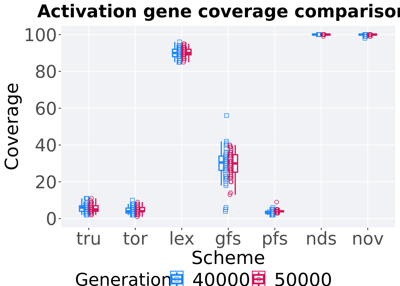
Best activation gene coverage in the population at 40,000 and 50,000 generations.

mvc_p = ggplot(mid, aes(x = acron, y=uni_str_pos, group = acron, shape = Generation)) +
  geom_point(col = mvc_col[1] , position = position_jitternudge(jitter.width = .03, nudge.x = -0.05), size = 2, alpha = 1.0) +
  geom_boxplot(position = position_nudge(x = -.15, y = 0), lwd = 0.7, col = mvc_col[1], fill = mvc_col[1], width = .1, outlier.shape = NA, alpha = 0.0) +

  geom_point(data = end, aes(x = acron, y=uni_str_pos), col = mvc_col[2], position = position_jitternudge(jitter.width = .03, nudge.x = 0.05), size = 2, alpha = 1.0) +
  geom_boxplot(data = end, aes(x = acron, y=uni_str_pos), position = position_nudge(x = .15, y = 0), lwd = 0.7, col = mvc_col[2], fill = mvc_col[2], width = .1, outlier.shape = NA, alpha = 0.0) +

  scale_y_continuous(
    name="Coverage",
    limits=c(0, 100),
    breaks=seq(0,100, 20),
    labels=c("0", "20", "40", "60", "80", "100")  ) +
  scale_x_discrete(
    name="Scheme"
  )+
  scale_shape_manual(values=c(0,1))+
  scale_colour_manual(values = c(mvc_col[1],mvc_col[2])) +
  p_theme

plot_grid(
  mvc_p +
    ggtitle("Activation gene coverage comparisons") +
    theme(legend.position="none"),
  legend,
  nrow=2,
  rel_heights = c(1,.05),
  label_size = TSIZE
)

4.5.2.3 Stats

Summary statistics for the activation gene coverage at 40,000 and 50,000 generations.

slices = filter(cc_over_time_mvc, diagnostic == 'contradictory_objectives' & (gen == 50000 | gen == 40000) & acron != 'ran')
slices$Generation <- factor(slices$gen, levels = c(50000,40000))
slices$acron = factor(slices$acron, levels = c('nov','nds','lex','gfs','tor','tru','pfs'))
slices %>%
  group_by(acron, Generation) %>%
  dplyr::summarise(
    count = n(),
    na_cnt = sum(is.na(uni_str_pos)),
    min = min(uni_str_pos, na.rm = TRUE),
    median = median(uni_str_pos, na.rm = TRUE),
    mean = mean(uni_str_pos, na.rm = TRUE),
    max = max(uni_str_pos, na.rm = TRUE),
    IQR = IQR(uni_str_pos, na.rm = TRUE)
  )

## `summarise()` has grouped output by 'acron'. You can override using the
## `.groups` argument.

## # A tibble: 14 x 9
## # Groups:   acron [7]
##    acron Generation count na_cnt   min median   mean   max   IQR
##    <fct> <fct>      <int>  <int> <int>  <dbl>  <dbl> <int> <dbl>
##  1 nov   50000         50      0    99  100   100.     100  0   
##  2 nov   40000         50      0    98  100    99.8    100  0   
##  3 nds   50000         50      0    99  100   100.     100  0   
##  4 nds   40000         50      0   100  100   100      100  0   
##  5 lex   50000         50      0    85   90    90.3     95  3   
##  6 lex   40000         50      0    85   90    90.0     96  4   
##  7 gfs   50000         50      0    13   30    29.4     40  9.5 
##  8 gfs   40000         50      0     4   30.5  29.3     56  7.75
##  9 tor   50000         50      0     1    4     4.64     9  2   
## 10 tor   40000         50      0     2    4     4.54    10  2.75
## 11 tru   50000         50      0     2    5     5.6     11  3   
## 12 tru   40000         50      0     2    6     5.8     11  3   
## 13 pfs   50000         50      0     3    4     4.02     9  0   
## 14 pfs   40000         50      0     2    3     3.42     6  1

Truncation selection comparisons.

wilcox.test(x = filter(slices, acron == 'tru' & Generation == 50000)$uni_str_pos,
            y = filter(slices, acron == 'tru' & Generation == 40000)$uni_str_pos,
            alternative = 't')

## 
##  Wilcoxon rank sum test with continuity correction
## 
## data:  filter(slices, acron == "tru" & Generation == 50000)$uni_str_pos and filter(slices, acron == "tru" & Generation == 40000)$uni_str_pos
## W = 1175, p-value = 0.6039
## alternative hypothesis: true location shift is not equal to 0

Tournament selection comparisons.

wilcox.test(x = filter(slices, acron == 'tor' & Generation == 50000)$uni_str_pos,
            y = filter(slices, acron == 'tor' & Generation == 40000)$uni_str_pos,
            alternative = 't')

## 
##  Wilcoxon rank sum test with continuity correction
## 
## data:  filter(slices, acron == "tor" & Generation == 50000)$uni_str_pos and filter(slices, acron == "tor" & Generation == 40000)$uni_str_pos
## W = 1351.5, p-value = 0.4781
## alternative hypothesis: true location shift is not equal to 0

Lexicase selection comparisons.

wilcox.test(x = filter(slices, acron == 'lex' & Generation == 50000)$uni_str_pos,
            y = filter(slices, acron == 'lex' & Generation == 40000)$uni_str_pos,
            alternative = 't')

## 
##  Wilcoxon rank sum test with continuity correction
## 
## data:  filter(slices, acron == "lex" & Generation == 50000)$uni_str_pos and filter(slices, acron == "lex" & Generation == 40000)$uni_str_pos
## W = 1321.5, p-value = 0.6221
## alternative hypothesis: true location shift is not equal to 0

Genotypic fitness sharing comparisons.

wilcox.test(x = filter(slices, acron == 'gfs' & Generation == 50000)$uni_str_pos,
            y = filter(slices, acron == 'gfs' & Generation == 40000)$uni_str_pos,
            alternative = 't')

## 
##  Wilcoxon rank sum test with continuity correction
## 
## data:  filter(slices, acron == "gfs" & Generation == 50000)$uni_str_pos and filter(slices, acron == "gfs" & Generation == 40000)$uni_str_pos
## W = 1223.5, p-value = 0.8575
## alternative hypothesis: true location shift is not equal to 0

Phenotypic fitness sharing comparisons.

wilcox.test(x = filter(slices, acron == 'pfs' & Generation == 50000)$uni_str_pos,
            y = filter(slices, acron == 'pfs' & Generation == 40000)$uni_str_pos,
            alternative = 't')

## 
##  Wilcoxon rank sum test with continuity correction
## 
## data:  filter(slices, acron == "pfs" & Generation == 50000)$uni_str_pos and filter(slices, acron == "pfs" & Generation == 40000)$uni_str_pos
## W = 1709, p-value = 0.0006733
## alternative hypothesis: true location shift is not equal to 0

Nondominated sorting comparisons.

wilcox.test(x = filter(slices, acron == 'nds' & Generation == 50000)$uni_str_pos,
            y = filter(slices, acron == 'nds' & Generation == 40000)$uni_str_pos,
            alternative = 't')

## 
##  Wilcoxon rank sum test with continuity correction
## 
## data:  filter(slices, acron == "nds" & Generation == 50000)$uni_str_pos and filter(slices, acron == "nds" & Generation == 40000)$uni_str_pos
## W = 1225, p-value = 0.3271
## alternative hypothesis: true location shift is not equal to 0

Novelty search comparisons.

wilcox.test(x = filter(slices, acron == 'nov' & Generation == 50000)$uni_str_pos,
            y = filter(slices, acron == 'nov' & Generation == 40000)$uni_str_pos,
            alternative = 't')

## 
##  Wilcoxon rank sum test with continuity correction
## 
## data:  filter(slices, acron == "nov" & Generation == 50000)$uni_str_pos and filter(slices, acron == "nov" & Generation == 40000)$uni_str_pos
## W = 1476, p-value = 0.007657
## alternative hypothesis: true location shift is not equal to 0