Chapter 3 Ordered exploitation results

Here we present the results for best performances found by each selection scheme replicate on the ordered exploitation diagnostic. Best performance found refers to the largest average trait score found in a given population. Note that performance values fall between 0.0 and 100.0.

3.1 Analysis dependencies

library(ggplot2)
library(cowplot)
library(dplyr)
library(PupillometryR)
library(sdamr)

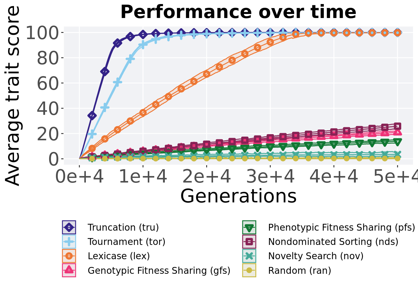
3.2 Performance over time

Best performance in a population over time.

# data for lines and shading on plots
lines = filter(cc_over_time, diagnostic == 'ordered_exploitation') %>%
  group_by(`Selection\nScheme`, gen) %>%
  dplyr::summarise(
    min = min(pop_fit_max) / DIMENSIONALITY,
    mean = mean(pop_fit_max) / DIMENSIONALITY,
    max = max(pop_fit_max) / DIMENSIONALITY
  )

## `summarise()` has grouped output by 'Selection Scheme'. You can override using
## the `.groups` argument.

ggplot(lines, aes(x=gen, y=mean, group = `Selection\nScheme`, fill =`Selection\nScheme`, color = `Selection\nScheme`, shape = `Selection\nScheme`)) +
  geom_ribbon(aes(ymin = min, ymax = max), alpha = 0.1) +
  geom_line(size = 0.5) +
  geom_point(data = filter(lines, gen %% 2000 == 0 & gen != 0), size = 1.5, stroke = 2.0, alpha = 1.0) +
  scale_y_continuous(
    name="Average trait score",
    limits=c(0, 100),
    breaks=seq(0,100, 20),
    labels=c("0", "20", "40", "60", "80", "100")
  ) +
  scale_x_continuous(
    name="Generations",
    limits=c(0, 50000),
    breaks=c(0, 10000, 20000, 30000, 40000, 50000),
    labels=c("0e+4", "1e+4", "2e+4", "3e+4", "4e+4", "5e+4")

  ) +
  scale_shape_manual(values=SHAPE)+
  scale_colour_manual(values = cb_palette) +
  scale_fill_manual(values = cb_palette) +
  ggtitle('Performance over time')+
  p_theme + theme(legend.title=element_blank(),legend.text=element_text(size=11)) +
  guides(
    shape=guide_legend(ncol=2, title.position = "bottom"),
    color=guide_legend(ncol=2, title.position = "bottom"),
    fill=guide_legend(ncol=2, title.position = "bottom")
  )

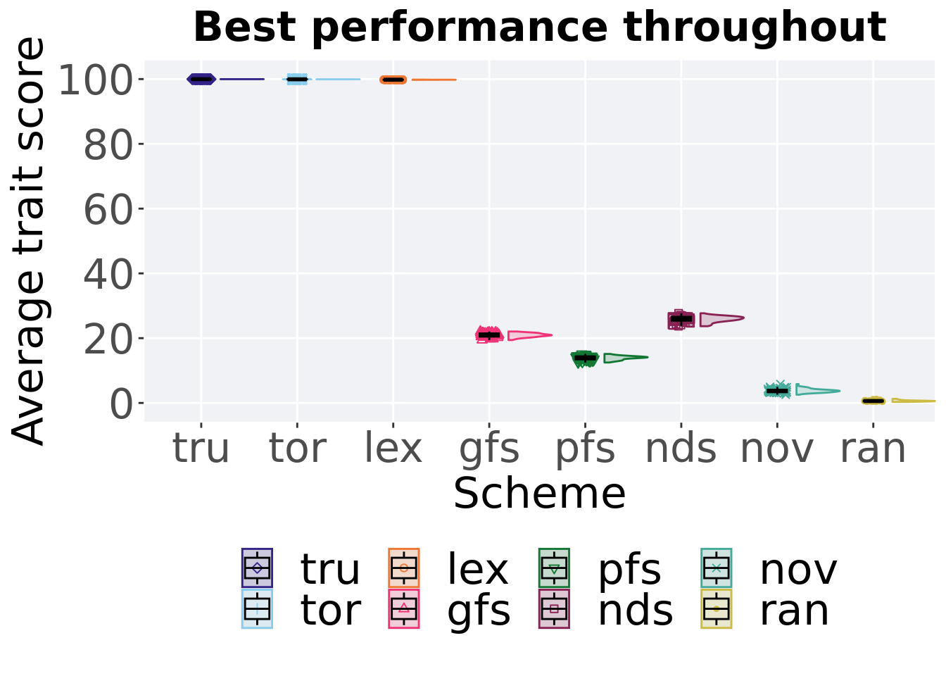
3.3 Best performance throughout

Best performance found throughout 50,000 generations.

### best performance throughout
filter(cc_best, col == 'pop_fit_max' & diagnostic == 'ordered_exploitation') %>%
  ggplot(., aes(x = acron, y = val / DIMENSIONALITY, color = acron, fill = acron, shape = acron)) +
  geom_flat_violin(position = position_nudge(x = .2, y = 0), scale = 'width', alpha = 0.2) +
  geom_point(position = position_jitter(width = .1), size = 1.5, alpha = 1.0) +
  geom_boxplot(color = 'black', width = .2, outlier.shape = NA, alpha = 0.0) +
  scale_y_continuous(
    name="Average trait score",
    limits=c(-1, 101),
    breaks=seq(0,100, 20),
    labels=c("0", "20", "40", "60", "80", "100")
  ) +
  scale_x_discrete(
    name="Scheme"
  )+
  scale_shape_manual(values=SHAPE)+
  scale_colour_manual(values = cb_palette, ) +
  scale_fill_manual(values = cb_palette) +
  ggtitle('Best performance throughout')+
  p_theme + theme(legend.title=element_blank()) +
  guides(
    shape=guide_legend(nrow=2, title.position = "bottom"),
    color=guide_legend(nrow=2, title.position = "bottom"),
    fill=guide_legend(nrow=2, title.position = "bottom")
  )

3.3.1 Stats

Summary statistics for the performance of the best performance throughout 50,000 generations.

#get data & summarize
performance = filter(cc_best, col == 'pop_fit_max' & diagnostic == 'ordered_exploitation')
performance$acron = factor(performance$acron, levels = c('tru', 'tor', 'lex','nds', 'gfs', 'pfs', 'nov',  'ran'))
performance %>%
  group_by(acron) %>%
  dplyr::summarise(
    count = n(),
    na_cnt = sum(is.na(val)),
    min = min(val / DIMENSIONALITY, na.rm = TRUE),
    median = median(val / DIMENSIONALITY, na.rm = TRUE),
    mean = mean(val / DIMENSIONALITY, na.rm = TRUE),
    max = max(val / DIMENSIONALITY, na.rm = TRUE),
    IQR = IQR(val / DIMENSIONALITY, na.rm = TRUE)
  )

## # A tibble: 8 x 8
##   acron count na_cnt     min  median    mean    max     IQR
##   <fct> <int>  <int>   <dbl>   <dbl>   <dbl>  <dbl>   <dbl>
## 1 tru      50      0 100.    100.    100.    100.   0.00208
## 2 tor      50      0  99.9    99.9    99.9    99.9  0.00445
## 3 lex      50      0  99.8    99.8    99.8    99.8  0.0207 
## 4 nds      50      0  23.7    26.0    25.9    27.7  1.17   
## 5 gfs      50      0  19.4    21.0    20.9    22.1  0.970  
## 6 pfs      50      0  12.5    14.1    13.9    15.1  0.871  
## 7 nov      50      0   2.55    3.70    3.80    5.82 0.718  
## 8 ran      50      0   0.319   0.598   0.634   1.26 0.240

Kruskal–Wallis test provides evidence of statistical differences.

kruskal.test(val ~ acron, data = performance)

## 
##  Kruskal-Wallis rank sum test
## 
## data:  val by acron
## Kruskal-Wallis chi-squared = 392.77, df = 7, p-value < 2.2e-16

Results for post-hoc Wilcoxon rank-sum test with a Bonferroni correction.

pairwise.wilcox.test(x = performance$val, g = performance$acron, p.adjust.method = "bonferroni",
                     paired = FALSE, conf.int = FALSE, alternative = 'l')

## 
##  Pairwise comparisons using Wilcoxon rank sum test with continuity correction 
## 
## data:  performance$val and performance$acron 
## 
##     tru    tor    lex    nds    gfs    pfs    nov   
## tor <2e-16 -      -      -      -      -      -     
## lex <2e-16 <2e-16 -      -      -      -      -     
## nds <2e-16 <2e-16 <2e-16 -      -      -      -     
## gfs <2e-16 <2e-16 <2e-16 <2e-16 -      -      -     
## pfs <2e-16 <2e-16 <2e-16 <2e-16 <2e-16 -      -     
## nov <2e-16 <2e-16 <2e-16 <2e-16 <2e-16 <2e-16 -     
## ran <2e-16 <2e-16 <2e-16 <2e-16 <2e-16 <2e-16 <2e-16
## 
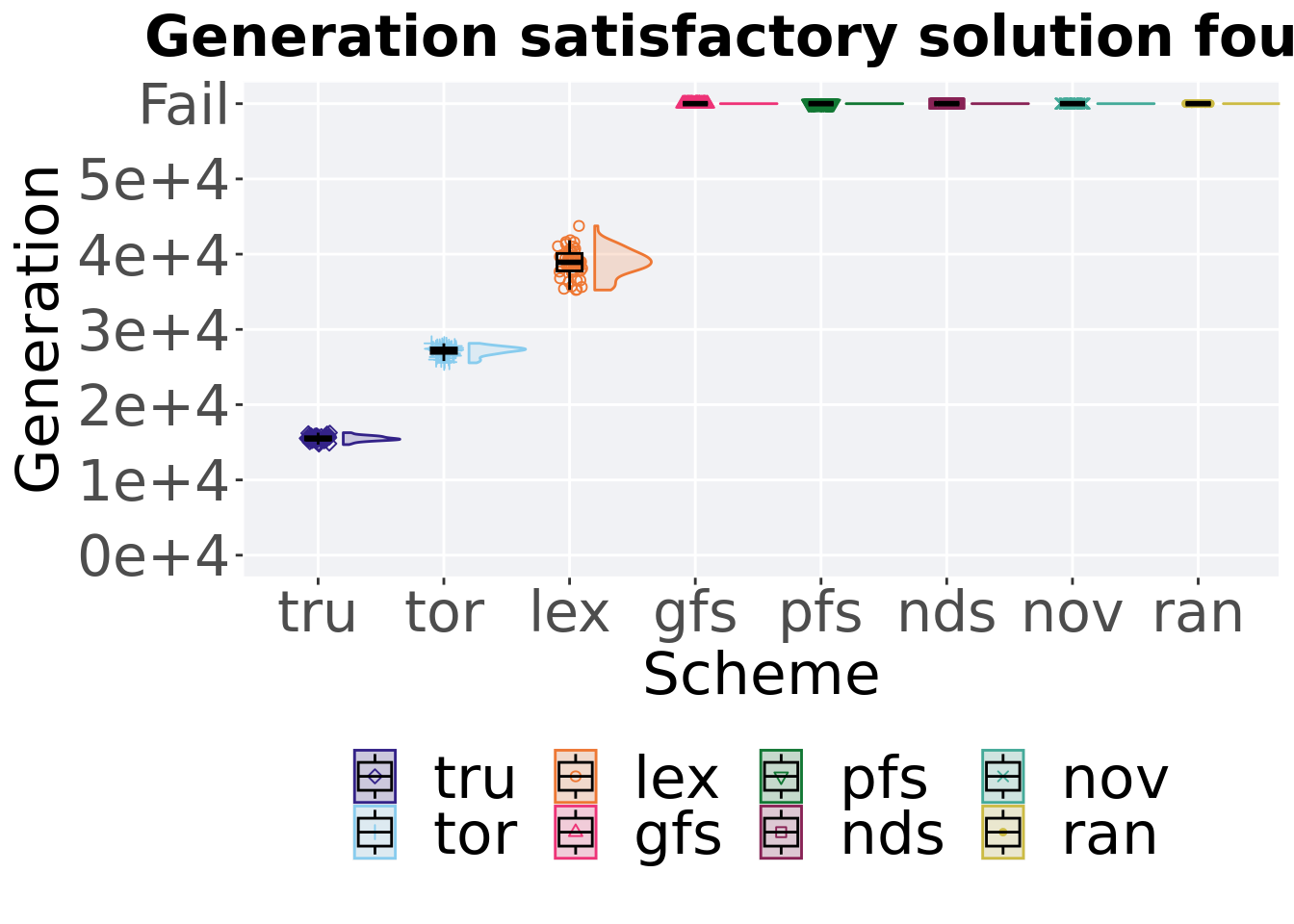
## P value adjustment method: bonferroni

3.4 Generation satisfactory solution found

First generation a satisfactory solution is found throughout the 50,000 generations.

### satisfactory solution found
filter(cc_ssf, diagnostic == 'ordered_exploitation') %>%
  ggplot(., aes(x = acron, y = Generations , color = acron, fill = acron, shape = acron)) +
  geom_flat_violin(position = position_nudge(x = .2, y = 0), scale = 'width', alpha = 0.2) +
  geom_point(position = position_jitter(width = .1), size = 1.5, alpha = 1.0) +
  geom_boxplot(color = 'black', width = .2, outlier.shape = NA, alpha = 0.0) +
  scale_y_continuous(
    name="Generation",
    limits=c(0, 60001),
    breaks=c(0, 10000, 20000, 30000, 40000, 50000, 60000),
    labels=c("0e+4", "1e+4", "2e+4", "3e+4", "4e+4", "5e+4", "Fail")
  ) +
  scale_x_discrete(
    name="Scheme"
  )+
  scale_shape_manual(values=SHAPE)+
  scale_colour_manual(values = cb_palette, ) +
  scale_fill_manual(values = cb_palette) +
  ggtitle('Generation satisfactory solution found')+
  p_theme + theme(legend.title=element_blank()) +
  guides(
    shape=guide_legend(nrow=2, title.position = "bottom"),
    color=guide_legend(nrow=2, title.position = "bottom"),
    fill=guide_legend(nrow=2, title.position = "bottom")
  )

3.4.1 Stats

Summary statistics for the first generation a satisfactory solution is found throughout the 50,000 generations.

### Generation satisfactory solution found
ssf = filter(cc_ssf, diagnostic == 'ordered_exploitation'  & Generations < 60000)
ssf$acron = factor(ssf$acron, levels = c('tru', 'tor', 'lex'))
ssf %>%
  group_by(acron) %>%
  dplyr::summarise(
    count = n(),
    na_cnt = sum(is.na(Generations)),
    min = min(Generations, na.rm = TRUE),
    median = median(Generations, na.rm = TRUE),
    mean = mean(Generations, na.rm = TRUE),
    max = max(Generations, na.rm = TRUE),
    IQR = IQR(Generations, na.rm = TRUE)
  )

## # A tibble: 3 x 8
##   acron count na_cnt   min median   mean   max   IQR
##   <fct> <int>  <int> <int>  <dbl>  <dbl> <int> <dbl>
## 1 tru      50      0 14701 15466. 15511. 16280  422.
## 2 tor      50      0 25563 27254. 27122. 28151  714 
## 3 lex      50      0 35240 38918. 38865. 43751 2316.

Kruskal–Wallis test provides evidence of difference amoung selection schemes.

kruskal.test(Generations ~ acron, data = ssf)

## 
##  Kruskal-Wallis rank sum test
## 
## data:  Generations by acron
## Kruskal-Wallis chi-squared = 132.45, df = 2, p-value < 2.2e-16

Results for post-hoc Wilcoxon rank-sum test with a Bonferroni correction.

pairwise.wilcox.test(x = ssf$Generations, g = ssf$acron, p.adjust.method = "bonferroni",
                     paired = FALSE, conf.int = FALSE, alternative = 'g')

## 
##  Pairwise comparisons using Wilcoxon rank sum test with continuity correction 
## 
## data:  ssf$Generations and ssf$acron 
## 
##     tru    tor   
## tor <2e-16 -     
## lex <2e-16 <2e-16
## 
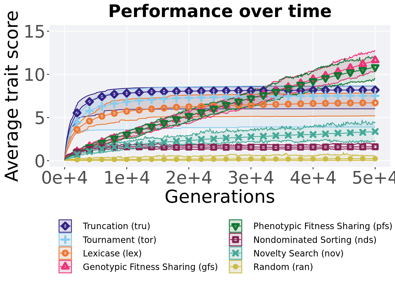
## P value adjustment method: bonferroni

3.5 Multi-valley crossing results

3.5.1 Performance over time

Best performance in a population over time.

# data for lines and shading on plots
lines = filter(cc_over_time_mvc, diagnostic == 'ordered_exploitation') %>%
  group_by(`Selection\nScheme`, gen) %>%
  dplyr::summarise(
    min = min(pop_fit_max) / DIMENSIONALITY,
    mean = mean(pop_fit_max) / DIMENSIONALITY,
    max = max(pop_fit_max) / DIMENSIONALITY
  )

## `summarise()` has grouped output by 'Selection Scheme'. You can override using
## the `.groups` argument.

ggplot(lines, aes(x=gen, y=mean, group = `Selection\nScheme`, fill =`Selection\nScheme`, color = `Selection\nScheme`, shape = `Selection\nScheme`)) +
  geom_ribbon(aes(ymin = min, ymax = max), alpha = 0.1) +
  geom_line(size = 0.5) +
  geom_point(data = filter(lines, gen %% 2000 == 0 & gen != 0), size = 1.5, stroke = 2.0, alpha = 1.0) +
  scale_y_continuous(
    name="Average trait score",
    limits=c(0, 15),
    breaks=seq(0,15, 5),
    labels=c("0", "5", "10", "15")
  ) +
  scale_x_continuous(
    name="Generations",
    limits=c(0, 50000),
    breaks=c(0, 10000, 20000, 30000, 40000, 50000),
    labels=c("0e+4", "1e+4", "2e+4", "3e+4", "4e+4", "5e+4")

  ) +
  scale_shape_manual(values=SHAPE)+
  scale_colour_manual(values = cb_palette) +
  scale_fill_manual(values = cb_palette) +
  ggtitle('Performance over time')+
  p_theme + theme(legend.title=element_blank(),legend.text=element_text(size=11)) +
  guides(
    shape=guide_legend(ncol=2, title.position = "left"),
    color=guide_legend(ncol=2, title.position = "left"),
    fill=guide_legend(ncol=2, title.position = "left")
  )

3.5.2 Best performance throughout

Best performance found throughout 50,000 generations.

### best performance throughout
filter(cc_best_mvc, col == 'pop_fit_max' & diagnostic == 'ordered_exploitation') %>%
  ggplot(., aes(x = acron, y = val / DIMENSIONALITY, color = acron, fill = acron, shape = acron)) +
  geom_flat_violin(position = position_nudge(x = .2, y = 0), scale = 'width', alpha = 0.2) +
  geom_point(position = position_jitter(width = .1), size = 1.5, alpha = 1.0) +
  geom_boxplot(color = 'black', width = .2, outlier.shape = NA, alpha = 0.0) +
  guides(fill = "none",color = 'none', shape = 'none') +
  scale_y_continuous(
    name="Average trait score",
    limits=c(0, 15),
    breaks=seq(0,15, 5),
    labels=c("0", "5", "10", "15")
  ) +
  scale_x_discrete(
    name="Scheme"
  )+
  scale_shape_manual(values=SHAPE)+
  scale_colour_manual(values = cb_palette, ) +
  scale_fill_manual(values = cb_palette) +
  ggtitle('Best performance throughout')+
  p_theme + theme(legend.title=element_blank()) +
  guides(
    shape=guide_legend(nrow=2, title.position = "bottom"),
    color=guide_legend(nrow=2, title.position = "bottom"),
    fill=guide_legend(nrow=2, title.position = "bottom")
  )

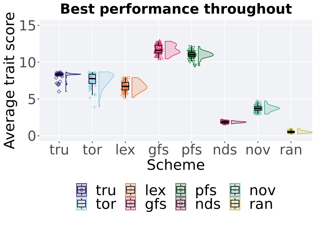
3.5.2.1 Stats

Summary statistics for the performance of the best performance.

#get data & summarize
performance = filter(cc_best_mvc, col == 'pop_fit_max' & diagnostic == 'ordered_exploitation')
performance$acron = factor(performance$acron, levels = c('gfs','pfs','tru','tor','lex','nov', 'nds', 'ran'))
performance %>%
  group_by(acron) %>%
  dplyr::summarise(
    count = n(),
    na_cnt = sum(is.na(val)),
    min = min(val / DIMENSIONALITY, na.rm = TRUE),
    median = median(val / DIMENSIONALITY, na.rm = TRUE),
    mean = mean(val / DIMENSIONALITY, na.rm = TRUE),
    max = max(val / DIMENSIONALITY, na.rm = TRUE),
    IQR = IQR(val / DIMENSIONALITY, na.rm = TRUE)
  )

## # A tibble: 8 x 8
##   acron count na_cnt    min median   mean    max    IQR
##   <fct> <int>  <int>  <dbl>  <dbl>  <dbl>  <dbl>  <dbl>
## 1 gfs      50      0 10.5   11.6   11.7   12.8   1.04  
## 2 pfs      50      0  9.54  11.0   11.0   12.1   0.553 
## 3 tru      50      0  6.01   8.35   8.19   8.65  0.0922
## 4 tor      50      0  3.91   7.76   7.52   8.68  1.26  
## 5 lex      50      0  5.20   6.70   6.72   7.91  1.01  
## 6 nov      50      0  2.95   3.71   3.72   4.73  0.476 
## 7 nds      50      0  1.63   1.86   1.85   2.09  0.129 
## 8 ran      50      0  0.263  0.490  0.534  0.968 0.202

Kruskal–Wallis test provides evidence of statistical differences.

kruskal.test(val ~ acron, data = performance)

## 
##  Kruskal-Wallis rank sum test
## 
## data:  val by acron
## Kruskal-Wallis chi-squared = 380.23, df = 7, p-value < 2.2e-16

Results for post-hoc Wilcoxon rank-sum test with a Bonferroni correction.

pairwise.wilcox.test(x = performance$val, g = performance$acron, p.adjust.method = "bonferroni",
                     paired = FALSE, conf.int = FALSE, alternative = 'l')

## 
##  Pairwise comparisons using Wilcoxon rank sum test with continuity correction 
## 
## data:  performance$val and performance$acron 
## 
##     gfs     pfs     tru     tor     lex     nov     nds    
## pfs 1.6e-06 -       -       -       -       -       -      
## tru < 2e-16 < 2e-16 -       -       -       -       -      
## tor < 2e-16 < 2e-16 0.0026  -       -       -       -      
## lex < 2e-16 < 2e-16 7.7e-14 1.7e-05 -       -       -      
## nov < 2e-16 < 2e-16 < 2e-16 2.4e-16 < 2e-16 -       -      
## nds < 2e-16 < 2e-16 < 2e-16 < 2e-16 < 2e-16 < 2e-16 -      
## ran < 2e-16 < 2e-16 < 2e-16 < 2e-16 < 2e-16 < 2e-16 < 2e-16
## 
## P value adjustment method: bonferroni

3.5.3 Performance comparison

Best performances in the population at 40,000 and 50,000 generations.

## Warning: The following aesthetics were dropped during statistical transformation:
## colour, shape
## i This can happen when ggplot fails to infer the correct grouping structure in
##   the data.
## i Did you forget to specify a `group` aesthetic or to convert a numerical
##   variable into a factor?
## The following aesthetics were dropped during statistical transformation:
## colour, shape
## i This can happen when ggplot fails to infer the correct grouping structure in
##   the data.
## i Did you forget to specify a `group` aesthetic or to convert a numerical
##   variable into a factor?

# 80% and final generation comparison
end = filter(cc_over_time_mvc, diagnostic == 'ordered_exploitation' & gen == 50000 & acron != 'ran')
end$Generation <- factor(end$gen)

mid = filter(cc_over_time_mvc, diagnostic == 'ordered_exploitation' & gen == 40000 & acron != 'ran')
mid$Generation <- factor(mid$gen)

mvc_p = ggplot(mid, aes(x = acron, y=pop_fit_max / DIMENSIONALITY, group = acron, shape = Generation)) +
  geom_point(col = mvc_col[1] , position = position_jitternudge(jitter.width = .03, nudge.x = -0.05), size = 2, alpha = 1.0) +
  geom_boxplot(position = position_nudge(x = -.15, y = 0), lwd = 0.7, col = mvc_col[1], fill = mvc_col[1], width = .1, outlier.shape = NA, alpha = 0.0) +

  geom_point(data = end, aes(x = acron, y=pop_fit_max / DIMENSIONALITY), col = mvc_col[2], position = position_jitternudge(jitter.width = .03, nudge.x = 0.05), size = 2, alpha = 1.0) +
  geom_boxplot(data = end, aes(x = acron, y=pop_fit_max / DIMENSIONALITY), position = position_nudge(x = .15, y = 0), lwd = 0.7, col = mvc_col[2], fill = mvc_col[2], width = .1, outlier.shape = NA, alpha = 0.0) +

  scale_y_continuous(
    name="Average trait score",
    limits=c(0, 15),
    breaks=seq(0,15, 5),
    labels=c("0", "5", "10", "15")
  ) +
  scale_x_discrete(
    name="Scheme"
  )+
  scale_shape_manual(values=c(0,1))+
  scale_colour_manual(values = c(mvc_col[1],mvc_col[2])) +
  p_theme

plot_grid(
  mvc_p +
    ggtitle("Performance comparisons") +
    theme(legend.position="none"),
  legend,
  nrow=2,
  rel_heights = c(1,.05),
  label_size = TSIZE
)

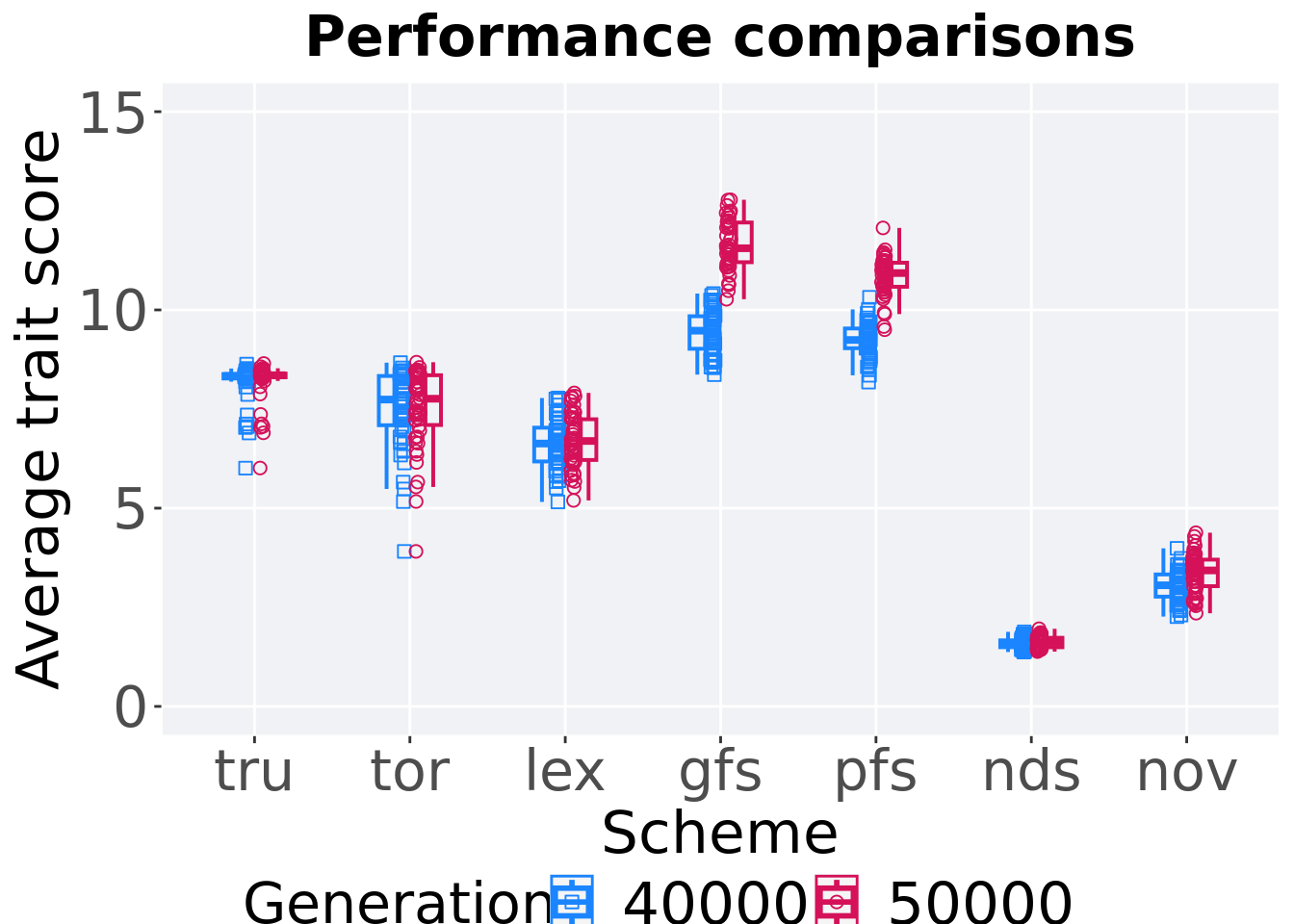
3.5.3.1 Stats

Summary statistics for the performance of the best performance at 40,000 and 50,000 generations.

### performance comparisons and generation slices 40K & 50K
slices = filter(cc_over_time_mvc, diagnostic == 'ordered_exploitation' & (gen == 50000 | gen == 40000) & acron != 'ran')
slices$Generation <- factor(slices$gen, levels = c(50000,40000))
slices$acron = factor(slices$acron, levels = c('gfs','pfs','tru','tor','lex','nov', 'nds', 'ran'))
slices %>%
  group_by(acron, Generation) %>%
  dplyr::summarise(
    count = n(),
    na_cnt = sum(is.na(pop_fit_max  / DIMENSIONALITY)),
    min = min(pop_fit_max  / DIMENSIONALITY, na.rm = TRUE),
    median = median(pop_fit_max  / DIMENSIONALITY, na.rm = TRUE),
    mean = mean(pop_fit_max  / DIMENSIONALITY, na.rm = TRUE),
    max = max(pop_fit_max  / DIMENSIONALITY, na.rm = TRUE),
    IQR = IQR(pop_fit_max  / DIMENSIONALITY, na.rm = TRUE)
  )

## `summarise()` has grouped output by 'acron'. You can override using the
## `.groups` argument.

## # A tibble: 14 x 9
## # Groups:   acron [7]
##    acron Generation count na_cnt   min median  mean   max    IQR
##    <fct> <fct>      <int>  <int> <dbl>  <dbl> <dbl> <dbl>  <dbl>
##  1 gfs   50000         50      0 10.3   11.6  11.6  12.8  1.00  
##  2 gfs   40000         50      0  8.37   9.48  9.45 10.4  0.820 
##  3 pfs   50000         50      0  9.50  10.9  10.8  12.1  0.606 
##  4 pfs   40000         50      0  8.18   9.24  9.23 10.3  0.498 
##  5 tru   50000         50      0  6.01   8.35  8.19  8.65 0.0922
##  6 tru   40000         50      0  6.01   8.33  8.17  8.63 0.112 
##  7 tor   50000         50      0  3.91   7.76  7.52  8.68 1.26  
##  8 tor   40000         50      0  3.91   7.74  7.49  8.67 1.24  
##  9 lex   50000         50      0  5.19   6.69  6.70  7.91 1.03  
## 10 lex   40000         50      0  5.16   6.63  6.63  7.78 0.852 
## 11 nov   50000         50      0  2.35   3.43  3.38  4.38 0.670 
## 12 nov   40000         50      0  2.27   3.06  3.03  3.99 0.560 
## 13 nds   50000         50      0  1.38   1.63  1.61  1.96 0.239 
## 14 nds   40000         50      0  1.37   1.58  1.58  1.88 0.173

Truncation selection comparisons.

wilcox.test(x = filter(slices, acron == 'tru' & Generation == 50000)$pop_fit_max,
            y = filter(slices, acron == 'tru' & Generation == 40000)$pop_fit_max,
            alternative = 't')

## 
##  Wilcoxon rank sum test with continuity correction
## 
## data:  filter(slices, acron == "tru" & Generation == 50000)$pop_fit_max and filter(slices, acron == "tru" & Generation == 40000)$pop_fit_max
## W = 1375, p-value = 0.3907
## alternative hypothesis: true location shift is not equal to 0

Tournament selection comparisons.

wilcox.test(x = filter(slices, acron == 'tor' & Generation == 50000)$pop_fit_max,
            y = filter(slices, acron == 'tor' & Generation == 40000)$pop_fit_max,
            alternative = 't')

## 
##  Wilcoxon rank sum test with continuity correction
## 
## data:  filter(slices, acron == "tor" & Generation == 50000)$pop_fit_max and filter(slices, acron == "tor" & Generation == 40000)$pop_fit_max
## W = 1306.5, p-value = 0.6995
## alternative hypothesis: true location shift is not equal to 0

Lexicase selection comparisons.

wilcox.test(x = filter(slices, acron == 'lex' & Generation == 50000)$pop_fit_max,
            y = filter(slices, acron == 'lex' & Generation == 40000)$pop_fit_max,
            alternative = 't')

## 
##  Wilcoxon rank sum test with continuity correction
## 
## data:  filter(slices, acron == "lex" & Generation == 50000)$pop_fit_max and filter(slices, acron == "lex" & Generation == 40000)$pop_fit_max
## W = 1348, p-value = 0.5015
## alternative hypothesis: true location shift is not equal to 0

Genotypic fitness sharing comparisons.

wilcox.test(x = filter(slices, acron == 'gfs' & Generation == 50000)$pop_fit_max,
            y = filter(slices, acron == 'gfs' & Generation == 40000)$pop_fit_max,
            alternative = 't')

## 
##  Wilcoxon rank sum test with continuity correction
## 
## data:  filter(slices, acron == "gfs" & Generation == 50000)$pop_fit_max and filter(slices, acron == "gfs" & Generation == 40000)$pop_fit_max
## W = 2498, p-value < 2.2e-16
## alternative hypothesis: true location shift is not equal to 0

Phenotypic fitness sharing comparisons.

wilcox.test(x = filter(slices, acron == 'pfs' & Generation == 50000)$pop_fit_max,
            y = filter(slices, acron == 'pfs' & Generation == 40000)$pop_fit_max,
            alternative = 't')

## 
##  Wilcoxon rank sum test with continuity correction
## 
## data:  filter(slices, acron == "pfs" & Generation == 50000)$pop_fit_max and filter(slices, acron == "pfs" & Generation == 40000)$pop_fit_max
## W = 2471, p-value < 2.2e-16
## alternative hypothesis: true location shift is not equal to 0

Nondominated sorting comparisons.

wilcox.test(x = filter(slices, acron == 'nds' & Generation == 50000)$pop_fit_max,
            y = filter(slices, acron == 'nds' & Generation == 40000)$pop_fit_max,
            alternative = 't')

## 
##  Wilcoxon rank sum test with continuity correction
## 
## data:  filter(slices, acron == "nds" & Generation == 50000)$pop_fit_max and filter(slices, acron == "nds" & Generation == 40000)$pop_fit_max
## W = 1413, p-value = 0.2626
## alternative hypothesis: true location shift is not equal to 0

Novelty search comparisons.

wilcox.test(x = filter(slices, acron == 'nov' & Generation == 50000)$pop_fit_max,
            y = filter(slices, acron == 'nov' & Generation == 40000)$pop_fit_max,
            alternative = 't')

## 
##  Wilcoxon rank sum test with continuity correction
## 
## data:  filter(slices, acron == "nov" & Generation == 50000)$pop_fit_max and filter(slices, acron == "nov" & Generation == 40000)$pop_fit_max
## W = 1789, p-value = 0.0002054
## alternative hypothesis: true location shift is not equal to 0