Chapter 8 Genotypic fitness sharing

We present the results from our parameter sweeep on genotypic fitness sharing. 50 replicates are conducted for each sigma parameter value explored. Note that when sigma = 0.0, no similarity penalty is used, and only stochastic remainder selection is used to identify parent solutions.

library(ggplot2)
library(cowplot)
library(dplyr)
library(PupillometryR)
library(sdamr)

8.1 Exploitation rate results

Here we present the results for best performances found by each genotypic fitness sharing sigma value replicate on the exploitation rate diagnostic. 50 replicates are conducted for each sigma parameter value explored. Note that when sigma = 0.0, no similarity penalty is used, and only stochastic remainder selection is used to identify parent solutions.

8.1.1 Performance over time

Performance over time.

lines =  filter(gfs_ot, diagnostic == 'exploitation_rate') %>%
  group_by(Sigma, gen) %>%
  dplyr::summarise(
    min = min(pop_fit_max),
    mean = mean(pop_fit_max),
    max = max(pop_fit_max)
  )

## `summarise()` has grouped output by 'Sigma'. You can override using the
## `.groups` argument.

ggplot(lines, aes(x=gen, y=mean / DIMENSIONALITY, group = Sigma, fill = Sigma, color = Sigma, shape = Sigma)) +
  geom_ribbon(aes(ymin = min / DIMENSIONALITY, ymax = max / DIMENSIONALITY), alpha = 0.1) +
  geom_line(size = 0.5) +
  geom_point(data = filter(lines, gen %% 2000 == 0 & gen != 0), size = 1.5, stroke = 2.0, alpha = 1.0) +
  scale_y_continuous(
    name="Average trait score"
  ) +
  scale_x_continuous(
    name="Generations",
    limits=c(0, 50000),
    breaks=c(0, 10000, 20000, 30000, 40000, 50000),
    labels=c("0e+4", "1e+4", "2e+4", "3e+4", "4e+4", "5e+4")

  ) +
  scale_shape_manual(values=SHAPE)+
  scale_colour_manual(values = cb_palette) +
  scale_fill_manual(values = cb_palette) +
  ggtitle("Best performance over time") +
  p_theme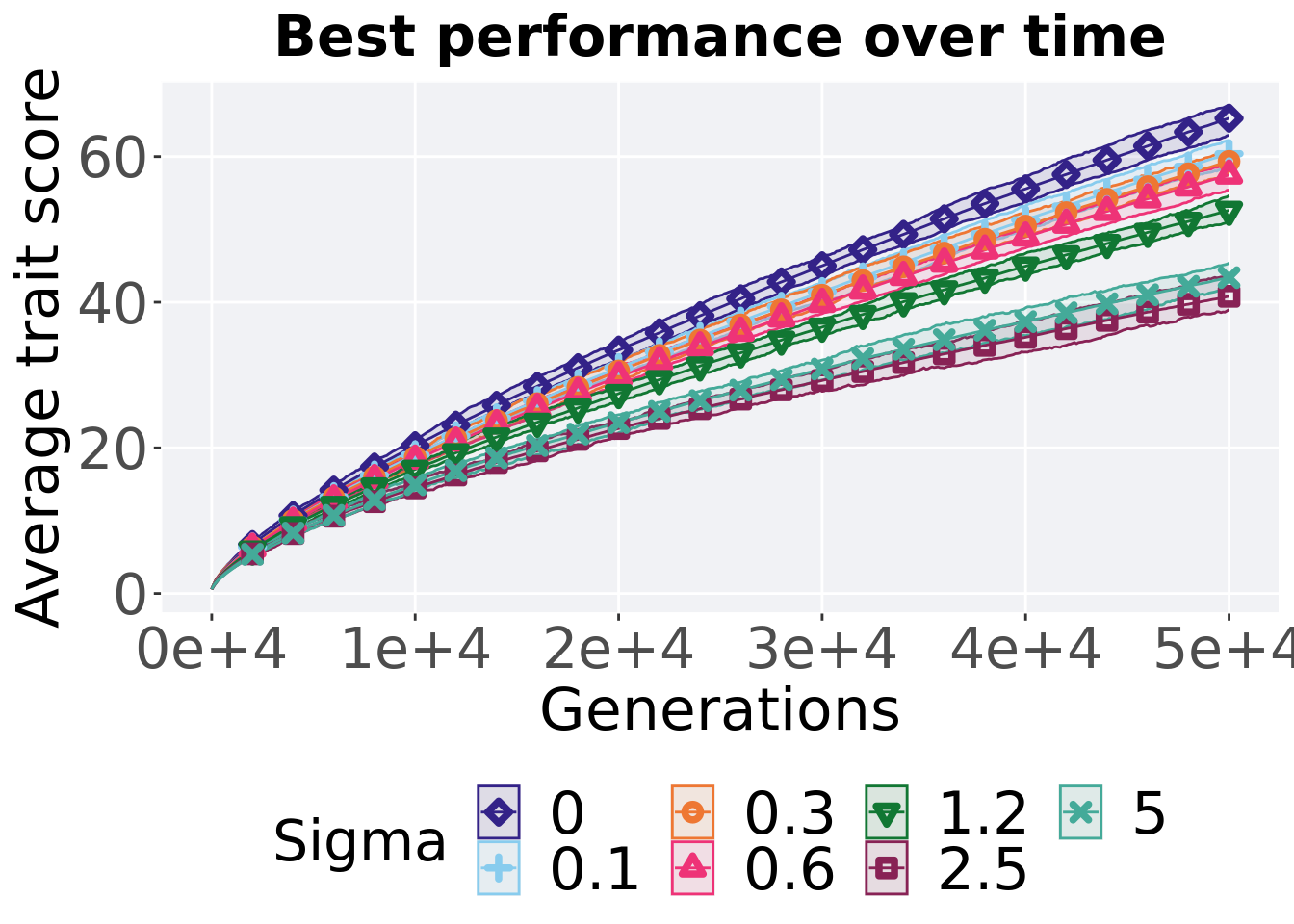

8.1.2 Best performance throughout

The best performance found throughout 50,000 generations.

filter(gfs_best, col == 'pop_fit_max' & diagnostic == 'exploitation_rate') %>%
ggplot(., aes(x = Sigma, y = val / DIMENSIONALITY, color = Sigma, fill = Sigma, shape = Sigma)) +
  geom_flat_violin(position = position_nudge(x = .2, y = 0), scale = 'width', alpha = 0.2) +
  geom_point(position = position_jitter(width = .1), size = 1.5, alpha = 1.0) +
  geom_boxplot(color = 'black', width = .2, outlier.shape = NA, alpha = 0.0) +
  scale_y_continuous(
    name="Average trait score",
    limits=c(-1, 80),
    breaks=seq(0,80, 20),
    labels=c("0", "20", "40", "60", "80")
  ) +
  scale_x_discrete(
    name="Sigma"
  )+
  scale_shape_manual(values=SHAPE)+
  scale_colour_manual(values = cb_palette) +
  scale_fill_manual(values = cb_palette) +
  ggtitle("Best performance throughout")+
  p_theme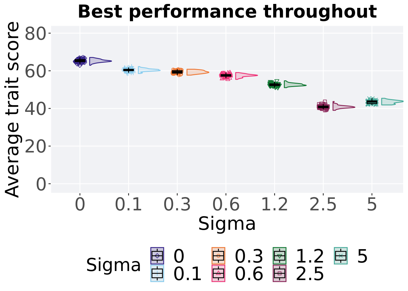

8.1.2.1 Stats

Summary statistics for the best performance found throughout 50,000 generations.

performance = filter(gfs_best, col == 'pop_fit_max' & diagnostic == 'exploitation_rate')
group_by(performance, Sigma) %>%
  dplyr::summarise(
    count = n(),
    na_cnt = sum(is.na(val)),
    min = min(val / DIMENSIONALITY, na.rm = TRUE),
    median = median(val / DIMENSIONALITY, na.rm = TRUE),
    mean = mean(val / DIMENSIONALITY, na.rm = TRUE),
    max = max(val / DIMENSIONALITY, na.rm = TRUE),
    IQR = IQR(val / DIMENSIONALITY, na.rm = TRUE)
  )

## # A tibble: 7 x 8
##   Sigma count na_cnt   min median  mean   max   IQR
##   <fct> <int>  <int> <dbl>  <dbl> <dbl> <dbl> <dbl>
## 1 0        50      0  62.9   65.3  65.3  67.1 1.11 
## 2 0.1      50      0  58.5   60.4  60.4  62.2 0.717
## 3 0.3      50      0  57.7   59.3  59.4  60.8 1.31 
## 4 0.6      50      0  55.4   57.6  57.5  59.1 0.843
## 5 1.2      50      0  51.1   52.5  52.6  54.7 0.907
## 6 2.5      50      0  39.0   40.8  40.9  43.7 0.813
## 7 5        50      0  41.9   43.6  43.4  45.4 1.43

Kruskal–Wallis test provides evidence of significant differences among sigma values on the best performance found throughout 50,000 generations

kruskal.test(val ~ Sigma,data = performance)

## 
##  Kruskal-Wallis rank sum test
## 
## data:  val by Sigma
## Kruskal-Wallis chi-squared = 336.49, df = 6, p-value < 2.2e-16

Results for post-hoc Wilcoxon rank-sum test with a Bonferroni correction on the best performance found throughout 50,000 generations.

pairwise.wilcox.test(x = performance$val, g = performance$Sigma , p.adjust.method = "bonferroni",
                     paired = FALSE, conf.int = FALSE, alternative = 'l')

## 
##  Pairwise comparisons using Wilcoxon rank sum test with continuity correction 
## 
## data:  performance$val and performance$Sigma 
## 
##     0       0.1     0.3     0.6     1.2     2.5
## 0.1 < 2e-16 -       -       -       -       -  
## 0.3 < 2e-16 1.5e-07 -       -       -       -  
## 0.6 < 2e-16 < 2e-16 3.0e-14 -       -       -  
## 1.2 < 2e-16 < 2e-16 < 2e-16 < 2e-16 -       -  
## 2.5 < 2e-16 < 2e-16 < 2e-16 < 2e-16 < 2e-16 -  
## 5   < 2e-16 < 2e-16 < 2e-16 < 2e-16 < 2e-16 1  
## 
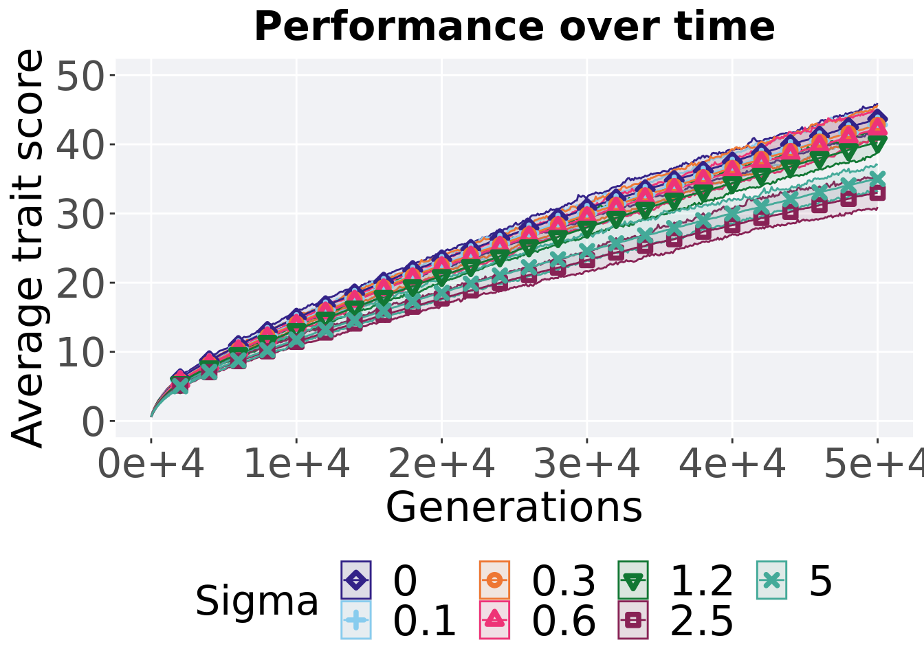
## P value adjustment method: bonferroni

8.1.3 Multi-valley crossing

8.1.3.1 Performance over time

# data for lines and shading on plots
lines = filter(gfs_ot_mvc, diagnostic == 'exploitation_rate') %>%
  group_by(Sigma, gen) %>%
  dplyr::summarise(
    min = min(pop_fit_max) / DIMENSIONALITY,
    mean = mean(pop_fit_max) / DIMENSIONALITY,
    max = max(pop_fit_max) / DIMENSIONALITY
  )

## `summarise()` has grouped output by 'Sigma'. You can override using the
## `.groups` argument.

ggplot(lines, aes(x=gen, y=mean, group = Sigma, fill =Sigma, color = Sigma, shape = Sigma)) +
  geom_ribbon(aes(ymin = min, ymax = max), alpha = 0.1) +
  geom_line(size = 0.5) +
  geom_point(data = filter(lines, gen %% 2000 == 0 & gen != 0), size = 1.5, stroke = 2.0, alpha = 1.0) +
  scale_y_continuous(
    name="Average trait score",
    limits=c(0, 50),
    breaks=seq(0,50, 10),
    labels=c("0", "10", "20", "30", "40", "50")
  ) +
  scale_x_continuous(
    name="Generations",
    limits=c(0, 50000),
    breaks=c(0, 10000, 20000, 30000, 40000, 50000),
    labels=c("0e+4", "1e+4", "2e+4", "3e+4", "4e+4", "5e+4")

  ) +
  scale_shape_manual(values=SHAPE)+
  scale_colour_manual(values = cb_palette) +
  scale_fill_manual(values = cb_palette) +
  ggtitle('Performance over time')+
  p_theme +
  guides(
    shape=guide_legend(nrow=2, title.position = "left"),
    color=guide_legend(nrow=2, title.position = "left"),
    fill=guide_legend(nrow=2, title.position = "left")
  )

8.1.3.2 Performance comparison

Best performances in the population at 40,000 and 50,000 generations.

## Warning: The following aesthetics were dropped during statistical transformation:
## colour, shape
## i This can happen when ggplot fails to infer the correct grouping structure in
##   the data.
## i Did you forget to specify a `group` aesthetic or to convert a numerical
##   variable into a factor?
## The following aesthetics were dropped during statistical transformation:
## colour, shape
## i This can happen when ggplot fails to infer the correct grouping structure in
##   the data.
## i Did you forget to specify a `group` aesthetic or to convert a numerical
##   variable into a factor?

# 80% and final generation comparison
end = filter(gfs_ot_mvc, diagnostic == 'exploitation_rate' & gen == 50000 & Sigma != 'ran')
end$Generation <- factor(end$gen)

mid = filter(gfs_ot_mvc, diagnostic == 'exploitation_rate' & gen == 40000 & Sigma != 'ran')
mid$Generation <- factor(mid$gen)

mvc_p = ggplot(mid, aes(x = Sigma, y=pop_fit_max / DIMENSIONALITY, group = Sigma, shape = Generation)) +
  geom_point(col = mvc_col[1] , position = position_jitternudge(jitter.width = .03, nudge.x = -0.05), size = 2, alpha = 1.0) +
  geom_boxplot(position = position_nudge(x = -.15, y = 0), lwd = 0.7, col = mvc_col[1], fill = mvc_col[1], width = .1, outlier.shape = NA, alpha = 0.0) +

  geom_point(data = end, aes(x = Sigma, y=pop_fit_max / DIMENSIONALITY), col = mvc_col[2], position = position_jitternudge(jitter.width = .03, nudge.x = 0.05), size = 2, alpha = 1.0) +
  geom_boxplot(data = end, aes(x = Sigma, y=pop_fit_max / DIMENSIONALITY), position = position_nudge(x = .15, y = 0), lwd = 0.7, col = mvc_col[2], fill = mvc_col[2], width = .1, outlier.shape = NA, alpha = 0.0) +

  scale_y_continuous(
    name="Average trait score",
    limits=c(0, 50),
    breaks=seq(0,50, 10),
    labels=c("0", "10", "20", "30", "40", "50")
  ) +
  scale_x_discrete(
    name="Sigma"
  )+
  scale_shape_manual(values=c(0,1))+
  scale_colour_manual(values = c(mvc_col[1],mvc_col[2])) +
  p_theme

plot_grid(
  mvc_p +
    ggtitle("Performance comparisons") +
    theme(legend.position="none"),
  legend,
  nrow=2,
  rel_heights = c(1,.05),
  label_size = TSIZE
)

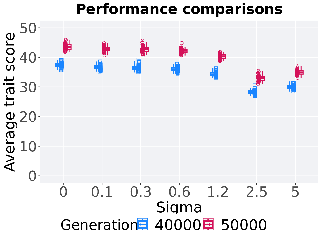
8.1.3.3 Stats

Summary statistics for the performance of the best performance at 40,000 and 50,000 generations.

slices = filter(gfs_ot_mvc, diagnostic == 'exploitation_rate' & (gen == 50000 | gen == 40000))
slices$Generation <- factor(slices$gen, levels = c(50000,40000))
slices %>%
  group_by(Sigma, Generation) %>%
  dplyr::summarise(
    count = n(),
    na_cnt = sum(is.na(pop_fit_max  / DIMENSIONALITY)),
    min = min(pop_fit_max  / DIMENSIONALITY, na.rm = TRUE),
    median = median(pop_fit_max  / DIMENSIONALITY, na.rm = TRUE),
    mean = mean(pop_fit_max  / DIMENSIONALITY, na.rm = TRUE),
    max = max(pop_fit_max  / DIMENSIONALITY, na.rm = TRUE),
    IQR = IQR(pop_fit_max  / DIMENSIONALITY, na.rm = TRUE)
  )

## `summarise()` has grouped output by 'Sigma'. You can override using the
## `.groups` argument.

## # A tibble: 14 x 9
## # Groups:   Sigma [7]
##    Sigma Generation count na_cnt   min median  mean   max   IQR
##    <fct> <fct>      <int>  <int> <dbl>  <dbl> <dbl> <dbl> <dbl>
##  1 0     50000         50      0  41.8   43.5  43.6  46.0 1.59 
##  2 0     40000         50      0  35.6   37.5  37.5  39.2 0.977
##  3 0.1   50000         50      0  40.7   42.7  42.8  44.9 1.10 
##  4 0.1   40000         50      0  35.2   36.8  36.7  38.6 1.14 
##  5 0.3   50000         50      0  40.7   42.8  42.8  45.7 1.21 
##  6 0.3   40000         50      0  34.9   36.4  36.6  39.3 1.15 
##  7 0.6   50000         50      0  40.6   42.3  42.2  44.8 1.24 
##  8 0.6   40000         50      0  34.3   36.0  36.1  37.9 1.18 
##  9 1.2   50000         50      0  38.8   40.4  40.3  41.9 1.49 
## 10 1.2   40000         50      0  33.2   34.3  34.4  36.3 1.16 
## 11 2.5   50000         50      0  30.9   32.9  33.0  35.4 1.37 
## 12 2.5   40000         50      0  27.0   28.4  28.3  30.7 1.07 
## 13 5     50000         50      0  33.1   34.9  35.0  37.0 1.17 
## 14 5     40000         50      0  28.5   29.9  30.0  31.9 0.977

Sigma 0.0

wilcox.test(x = filter(slices, Sigma == 0.0 & Generation == 50000)$pop_fit_max,
            y = filter(slices, Sigma == 0.0 & Generation == 40000)$pop_fit_max,
            alternative = 't')

## 
##  Wilcoxon rank sum test with continuity correction
## 
## data:  filter(slices, Sigma == 0 & Generation == 50000)$pop_fit_max and filter(slices, Sigma == 0 & Generation == 40000)$pop_fit_max
## W = 2500, p-value < 2.2e-16
## alternative hypothesis: true location shift is not equal to 0

Sigma 0.1

wilcox.test(x = filter(slices, Sigma == 0.1 & Generation == 50000)$pop_fit_max,
            y = filter(slices, Sigma == 0.1 & Generation == 40000)$pop_fit_max,
            alternative = 't')

## 
##  Wilcoxon rank sum test with continuity correction
## 
## data:  filter(slices, Sigma == 0.1 & Generation == 50000)$pop_fit_max and filter(slices, Sigma == 0.1 & Generation == 40000)$pop_fit_max
## W = 2500, p-value < 2.2e-16
## alternative hypothesis: true location shift is not equal to 0

Sigma 0.3

wilcox.test(x = filter(slices, Sigma == 0.3 & Generation == 50000)$pop_fit_max,
            y = filter(slices, Sigma == 0.3 & Generation == 40000)$pop_fit_max,
            alternative = 't')

## 
##  Wilcoxon rank sum test with continuity correction
## 
## data:  filter(slices, Sigma == 0.3 & Generation == 50000)$pop_fit_max and filter(slices, Sigma == 0.3 & Generation == 40000)$pop_fit_max
## W = 2500, p-value < 2.2e-16
## alternative hypothesis: true location shift is not equal to 0

Sigma 0.6

wilcox.test(x = filter(slices, Sigma == 0.6 & Generation == 50000)$pop_fit_max,
            y = filter(slices, Sigma == 0.6 & Generation == 40000)$pop_fit_max,
            alternative = 't')

## 
##  Wilcoxon rank sum test with continuity correction
## 
## data:  filter(slices, Sigma == 0.6 & Generation == 50000)$pop_fit_max and filter(slices, Sigma == 0.6 & Generation == 40000)$pop_fit_max
## W = 2500, p-value < 2.2e-16
## alternative hypothesis: true location shift is not equal to 0

Sigma 1.2

wilcox.test(x = filter(slices, Sigma == 1.2 & Generation == 50000)$pop_fit_max,
            y = filter(slices, Sigma == 1.2 & Generation == 40000)$pop_fit_max,
            alternative = 't')

## 
##  Wilcoxon rank sum test with continuity correction
## 
## data:  filter(slices, Sigma == 1.2 & Generation == 50000)$pop_fit_max and filter(slices, Sigma == 1.2 & Generation == 40000)$pop_fit_max
## W = 2500, p-value < 2.2e-16
## alternative hypothesis: true location shift is not equal to 0

Sigma 2.5

wilcox.test(x = filter(slices, Sigma == 2.5 & Generation == 50000)$pop_fit_max,
            y = filter(slices, Sigma == 2.5 & Generation == 40000)$pop_fit_max,
            alternative = 't')

## 
##  Wilcoxon rank sum test with continuity correction
## 
## data:  filter(slices, Sigma == 2.5 & Generation == 50000)$pop_fit_max and filter(slices, Sigma == 2.5 & Generation == 40000)$pop_fit_max
## W = 2500, p-value < 2.2e-16
## alternative hypothesis: true location shift is not equal to 0

Sigma 5.0

wilcox.test(x = filter(slices, Sigma == 5.0 & Generation == 50000)$pop_fit_max,
            y = filter(slices, Sigma == 5.0 & Generation == 40000)$pop_fit_max,
            alternative = 't')

## 
##  Wilcoxon rank sum test with continuity correction
## 
## data:  filter(slices, Sigma == 5 & Generation == 50000)$pop_fit_max and filter(slices, Sigma == 5 & Generation == 40000)$pop_fit_max
## W = 2500, p-value < 2.2e-16
## alternative hypothesis: true location shift is not equal to 0

8.2 Ordered exploitation results

Here we present the results for best performances found by each genotypic fitness sharing sigma value replicate on the ordered exploitation diagnostic. Best performance found refers to the largest average trait score found in a given population. Note that performance values fall between 0 and 100.

8.2.1 Performance over time

Performance over time.

lines =  filter(gfs_ot, diagnostic == 'ordered_exploitation') %>%
  group_by(Sigma, gen) %>%
  dplyr::summarise(
    min = min(pop_fit_max),
    mean = mean(pop_fit_max),
    max = max(pop_fit_max)
  )

## `summarise()` has grouped output by 'Sigma'. You can override using the
## `.groups` argument.

ggplot(lines, aes(x=gen, y=mean / DIMENSIONALITY, group = Sigma, fill = Sigma, color = Sigma, shape = Sigma)) +
  geom_ribbon(aes(ymin = min / DIMENSIONALITY, ymax = max / DIMENSIONALITY), alpha = 0.1) +
  geom_line(size = 0.5) +
  geom_point(data = filter(lines, gen %% 2000 == 0 & gen != 0), size = 1.5, stroke = 2.0, alpha = 1.0) +
  scale_y_continuous(
    name="Average trait score"
  ) +
  scale_x_continuous(
    name="Generations",
    limits=c(0, 50000),
    breaks=c(0, 10000, 20000, 30000, 40000, 50000),
    labels=c("0e+4", "1e+4", "2e+4", "3e+4", "4e+4", "5e+4")

  ) +
  scale_shape_manual(values=SHAPE)+
  scale_colour_manual(values = cb_palette) +
  scale_fill_manual(values = cb_palette) +
  ggtitle("Best performance over time") +
  p_theme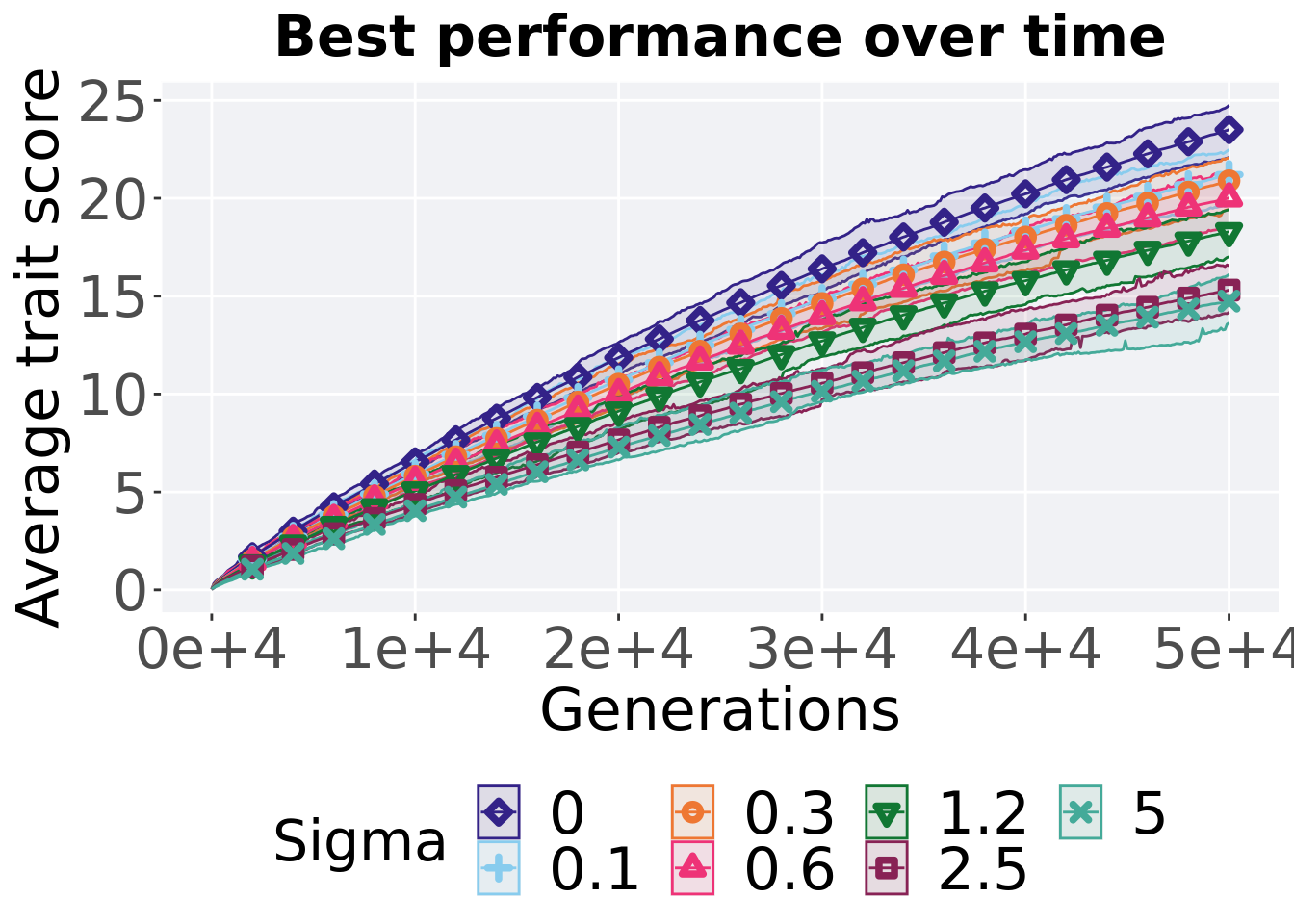

8.2.2 Best performance throughout

The best performance found throughout 50,000 generations.

filter(gfs_best, col == 'pop_fit_max' & diagnostic == 'ordered_exploitation') %>%
  ggplot(., aes(x = Sigma, y = val / DIMENSIONALITY, color = Sigma, fill = Sigma, shape = Sigma)) +
  geom_flat_violin(position = position_nudge(x = .2, y = 0), scale = 'width', alpha = 0.2) +
  geom_point(position = position_jitter(width = .1), size = 1.5, alpha = 1.0) +
  geom_boxplot(color = 'black', width = .2, outlier.shape = NA, alpha = 0.0) +
  scale_y_continuous(
    name="Average trait score"
  ) +
  scale_x_discrete(
    name="Sigma"
  )+
  scale_shape_manual(values=SHAPE)+
  scale_colour_manual(values = cb_palette) +
  scale_fill_manual(values = cb_palette) +
  ggtitle("Best performance throughout")+
  p_theme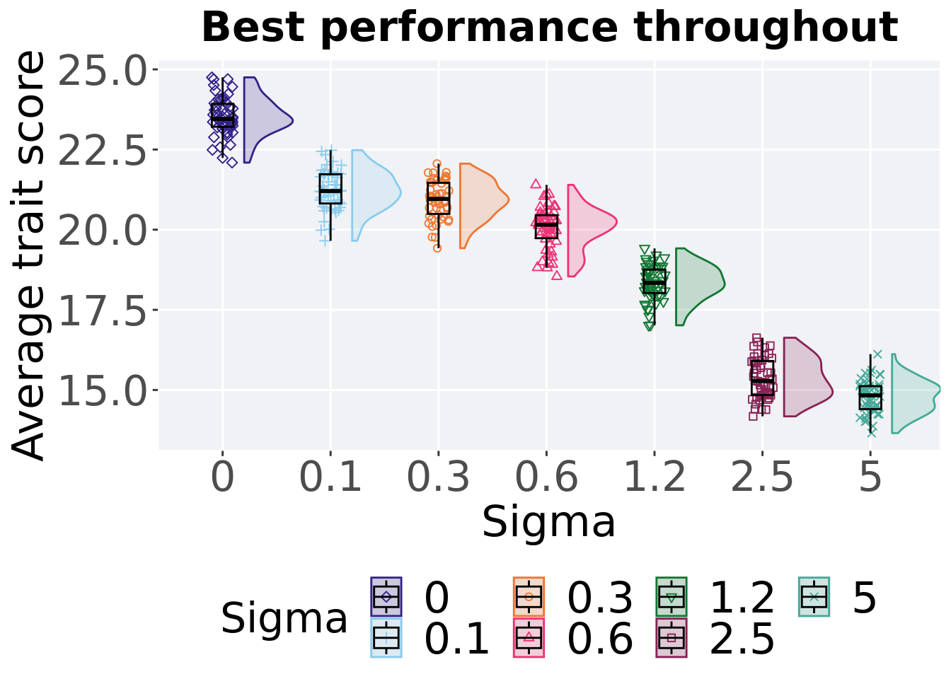

8.2.2.1 Stats

Summary statistics about the best performance found.

performance = filter(gfs_best, col == 'pop_fit_max' & diagnostic == 'ordered_exploitation')
group_by(performance, Sigma) %>%
  dplyr::summarise(
    count = n(),
    na_cnt = sum(is.na(val)),
    min = min(val / DIMENSIONALITY, na.rm = TRUE),
    median = median(val / DIMENSIONALITY, na.rm = TRUE),
    mean = mean(val / DIMENSIONALITY, na.rm = TRUE),
    max = max(val / DIMENSIONALITY, na.rm = TRUE),
    IQR = IQR(val / DIMENSIONALITY, na.rm = TRUE)
  )

## # A tibble: 7 x 8
##   Sigma count na_cnt   min median  mean   max   IQR
##   <fct> <int>  <int> <dbl>  <dbl> <dbl> <dbl> <dbl>
## 1 0        50      0  22.1   23.5  23.5  24.8 0.713
## 2 0.1      50      0  19.7   21.2  21.2  22.5 0.911
## 3 0.3      50      0  19.4   21.0  20.9  22.1 0.970
## 4 0.6      50      0  18.5   20.2  20.0  21.4 0.716
## 5 1.2      50      0  17.0   18.3  18.3  19.4 0.729
## 6 2.5      50      0  14.2   15.3  15.4  16.6 1.06 
## 7 5        50      0  13.7   14.8  14.8  16.1 0.717

Kruskal–Wallis test provides evidence of statistical differences for the best performance found in the pouplation throughout 50,000 generations.

kruskal.test(val ~ Sigma,data = performance)

## 
##  Kruskal-Wallis rank sum test
## 
## data:  val by Sigma
## Kruskal-Wallis chi-squared = 322.96, df = 6, p-value < 2.2e-16

Results for post-hoc Wilcoxon rank-sum test with a Bonferroni correction on the best performance found in the pouplation throughout 50,000 generations.

pairwise.wilcox.test(x = performance$val, g = performance$Sigma , p.adjust.method = "bonferroni",
                     paired = FALSE, conf.int = FALSE, alternative = 'l')

## 
##  Pairwise comparisons using Wilcoxon rank sum test with continuity correction 
## 
## data:  performance$val and performance$Sigma 
## 
##     0       0.1     0.3     0.6     1.2     2.5    
## 0.1 < 2e-16 -       -       -       -       -      
## 0.3 < 2e-16 0.15850 -       -       -       -      
## 0.6 < 2e-16 1.5e-11 5.6e-08 -       -       -      
## 1.2 < 2e-16 < 2e-16 < 2e-16 3.4e-15 -       -      
## 2.5 < 2e-16 < 2e-16 < 2e-16 < 2e-16 < 2e-16 -      
## 5   < 2e-16 < 2e-16 < 2e-16 < 2e-16 < 2e-16 0.00038
## 
## P value adjustment method: bonferroni

8.2.3 Multi-valley crossing

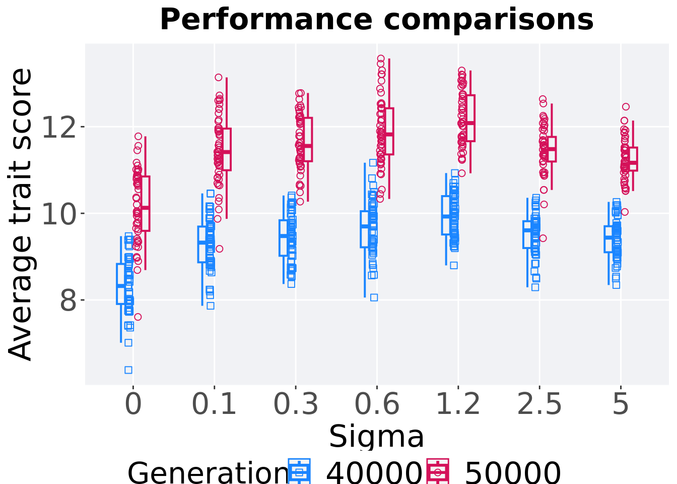
8.2.3.1 Performance comparison

Best performances in the population at 40,000 and 50,000 generations.

# 80% and final generation comparison
end = filter(gfs_ot_mvc, diagnostic == 'ordered_exploitation' & gen == 50000)
end$Generation <- factor(end$gen)

mid = filter(gfs_ot_mvc, diagnostic == 'ordered_exploitation' & gen == 40000)
mid$Generation <- factor(mid$gen)

mvc_p = ggplot(mid, aes(x = Sigma, y=pop_fit_max / DIMENSIONALITY, group = Sigma, shape = Generation)) +
  geom_point(col = mvc_col[1] , position = position_jitternudge(jitter.width = .03, nudge.x = -0.05), size = 2, alpha = 1.0) +
  geom_boxplot(position = position_nudge(x = -.15, y = 0), lwd = 0.7, col = mvc_col[1], fill = mvc_col[1], width = .1, outlier.shape = NA, alpha = 0.0) +

  geom_point(data = end, aes(x = Sigma, y=pop_fit_max / DIMENSIONALITY), col = mvc_col[2], position = position_jitternudge(jitter.width = .03, nudge.x = 0.05), size = 2, alpha = 1.0) +
  geom_boxplot(data = end, aes(x = Sigma, y=pop_fit_max / DIMENSIONALITY), position = position_nudge(x = .15, y = 0), lwd = 0.7, col = mvc_col[2], fill = mvc_col[2], width = .1, outlier.shape = NA, alpha = 0.0) +

  scale_y_continuous(
    name="Average trait score"
  ) +
  scale_x_discrete(
    name="Sigma"
  )+
  scale_shape_manual(values=c(0,1))+
  scale_colour_manual(values = c(mvc_col[1],mvc_col[2])) +
  p_theme

plot_grid(
  mvc_p +
    ggtitle("Performance comparisons") +
    theme(legend.position="none"),
  legend,
  nrow=2,
  rel_heights = c(1,.05),
  label_size = TSIZE
)

8.2.3.1.1 Stats

Summary statistics for the performance of the best performance at 40,000 and 50,000 generations.

slices = filter(gfs_ot_mvc, diagnostic == 'ordered_exploitation' & (gen == 50000 | gen == 40000))
slices$Generation <- factor(slices$gen, levels = c(50000,40000))
slices %>%
  group_by(Sigma, Generation) %>%
  dplyr::summarise(
    count = n(),
    na_cnt = sum(is.na(pop_fit_max  / DIMENSIONALITY)),
    min = min(pop_fit_max  / DIMENSIONALITY, na.rm = TRUE),
    median = median(pop_fit_max  / DIMENSIONALITY, na.rm = TRUE),
    mean = mean(pop_fit_max  / DIMENSIONALITY, na.rm = TRUE),
    max = max(pop_fit_max  / DIMENSIONALITY, na.rm = TRUE),
    IQR = IQR(pop_fit_max  / DIMENSIONALITY, na.rm = TRUE)
  )

## `summarise()` has grouped output by 'Sigma'. You can override using the
## `.groups` argument.

## # A tibble: 14 x 9
## # Groups:   Sigma [7]
##    Sigma Generation count na_cnt   min median  mean   max   IQR
##    <fct> <fct>      <int>  <int> <dbl>  <dbl> <dbl> <dbl> <dbl>
##  1 0     50000         50      0  7.61  10.1  10.2  11.8  1.26 
##  2 0     40000         50      0  6.38   8.32  8.31  9.47 0.924
##  3 0.1   50000         50      0  9.18  11.4  11.5  13.1  0.962
##  4 0.1   40000         50      0  7.86   9.32  9.28 10.5  0.825
##  5 0.3   50000         50      0 10.3   11.6  11.6  12.8  1.00 
##  6 0.3   40000         50      0  8.37   9.48  9.45 10.4  0.820
##  7 0.6   50000         50      0 10.3   11.8  11.9  13.6  1.07 
##  8 0.6   40000         50      0  8.06   9.70  9.64 11.2  0.833
##  9 1.2   50000         50      0 10.9   12.1  12.2  13.3  1.06 
## 10 1.2   40000         50      0  8.80   9.93  9.94 10.9  0.886
## 11 2.5   50000         50      0  9.42  11.5  11.4  12.6  0.568
## 12 2.5   40000         50      0  8.29   9.61  9.52 10.4  0.619
## 13 5     50000         50      0 10.0   11.2  11.2  12.5  0.533
## 14 5     40000         50      0  8.35   9.44  9.41 10.3  0.600

Sigma 0.0

wilcox.test(x = filter(slices, Sigma == 0.0 & Generation == 50000)$pop_fit_max,
            y = filter(slices, Sigma == 0.0 & Generation == 40000)$pop_fit_max,
            alternative = 't')

## 
##  Wilcoxon rank sum test with continuity correction
## 
## data:  filter(slices, Sigma == 0 & Generation == 50000)$pop_fit_max and filter(slices, Sigma == 0 & Generation == 40000)$pop_fit_max
## W = 2385, p-value = 5.239e-15
## alternative hypothesis: true location shift is not equal to 0

Sigma 0.1

wilcox.test(x = filter(slices, Sigma == 0.1 & Generation == 50000)$pop_fit_max,
            y = filter(slices, Sigma == 0.1 & Generation == 40000)$pop_fit_max,
            alternative = 't')

## 
##  Wilcoxon rank sum test with continuity correction
## 
## data:  filter(slices, Sigma == 0.1 & Generation == 50000)$pop_fit_max and filter(slices, Sigma == 0.1 & Generation == 40000)$pop_fit_max
## W = 2453, p-value < 2.2e-16
## alternative hypothesis: true location shift is not equal to 0

Sigma 0.3

wilcox.test(x = filter(slices, Sigma == 0.3 & Generation == 50000)$pop_fit_max,
            y = filter(slices, Sigma == 0.3 & Generation == 40000)$pop_fit_max,
            alternative = 't')

## 
##  Wilcoxon rank sum test with continuity correction
## 
## data:  filter(slices, Sigma == 0.3 & Generation == 50000)$pop_fit_max and filter(slices, Sigma == 0.3 & Generation == 40000)$pop_fit_max
## W = 2498, p-value < 2.2e-16
## alternative hypothesis: true location shift is not equal to 0

Sigma 0.6

wilcox.test(x = filter(slices, Sigma == 0.6 & Generation == 50000)$pop_fit_max,
            y = filter(slices, Sigma == 0.6 & Generation == 40000)$pop_fit_max,
            alternative = 't')

## 
##  Wilcoxon rank sum test with continuity correction
## 
## data:  filter(slices, Sigma == 0.6 & Generation == 50000)$pop_fit_max and filter(slices, Sigma == 0.6 & Generation == 40000)$pop_fit_max
## W = 2481, p-value < 2.2e-16
## alternative hypothesis: true location shift is not equal to 0

Sigma 1.2

wilcox.test(x = filter(slices, Sigma == 1.2 & Generation == 50000)$pop_fit_max,
            y = filter(slices, Sigma == 1.2 & Generation == 40000)$pop_fit_max,
            alternative = 't')

## 
##  Wilcoxon rank sum test with continuity correction
## 
## data:  filter(slices, Sigma == 1.2 & Generation == 50000)$pop_fit_max and filter(slices, Sigma == 1.2 & Generation == 40000)$pop_fit_max
## W = 2499, p-value < 2.2e-16
## alternative hypothesis: true location shift is not equal to 0

Sigma 2.5

wilcox.test(x = filter(slices, Sigma == 2.5 & Generation == 50000)$pop_fit_max,
            y = filter(slices, Sigma == 2.5 & Generation == 40000)$pop_fit_max,
            alternative = 't')

## 
##  Wilcoxon rank sum test with continuity correction
## 
## data:  filter(slices, Sigma == 2.5 & Generation == 50000)$pop_fit_max and filter(slices, Sigma == 2.5 & Generation == 40000)$pop_fit_max
## W = 2464, p-value < 2.2e-16
## alternative hypothesis: true location shift is not equal to 0

Sigma 5.0

wilcox.test(x = filter(slices, Sigma == 5.0 & Generation == 50000)$pop_fit_max,
            y = filter(slices, Sigma == 5.0 & Generation == 40000)$pop_fit_max,
            alternative = 't')

## 
##  Wilcoxon rank sum test with continuity correction
## 
## data:  filter(slices, Sigma == 5 & Generation == 50000)$pop_fit_max and filter(slices, Sigma == 5 & Generation == 40000)$pop_fit_max
## W = 2494, p-value < 2.2e-16
## alternative hypothesis: true location shift is not equal to 0

8.3 Contraditory objectives diagnostic

Here we present the results for satisfactory trait coverage and activation gene coverage found by each genotypic fitness sharing sigma value replicate on the ordered exploitation diagnostic. Satisfactory trait coverage refers to the count of unique satisfied DIMENSIONALITY in the population, while activation gene coverage refers to the count of unique activation genes in the population. Note that both coverage values fall between 0 and 100.

8.3.1 Satisfactory trait coverage

Satisfactory trait coverage analysis.

8.3.1.1 Coverage over time

Satisfactory trait coverage over time.

lines = filter(gfs_ot, diagnostic == 'contradictory_objectives') %>%
  group_by(Sigma, gen) %>%
  dplyr::summarise(
    min = min(pop_uni_obj),
    mean = mean(pop_uni_obj),
    max = max(pop_uni_obj)
  )

## `summarise()` has grouped output by 'Sigma'. You can override using the
## `.groups` argument.

ggplot(lines, aes(x=gen, y=mean, group = Sigma, fill =Sigma, color = Sigma, shape = Sigma)) +
  geom_ribbon(aes(ymin = min, ymax = max), alpha = 0.1) +
  geom_line(size = 0.5) +
  geom_point(data = filter(lines, gen %% 2000 == 0 & gen != 0), size = 1.5, stroke = 2.0, alpha = 1.0) +
  scale_y_continuous(
    name="Coverage",
    limits=c(0, 5)
  ) +
  scale_x_continuous(
    name="Generations",
    limits=c(0, 50000),
    breaks=c(0, 10000, 20000, 30000, 40000, 50000),
    labels=c("0e+4", "1e+4", "2e+4", "3e+4", "4e+4", "5e+4")

  ) +
  scale_shape_manual(values=SHAPE)+
  scale_colour_manual(values = cb_palette) +
  scale_fill_manual(values = cb_palette) +
  ggtitle("Satisfactory trait coverage over time") +
  p_theme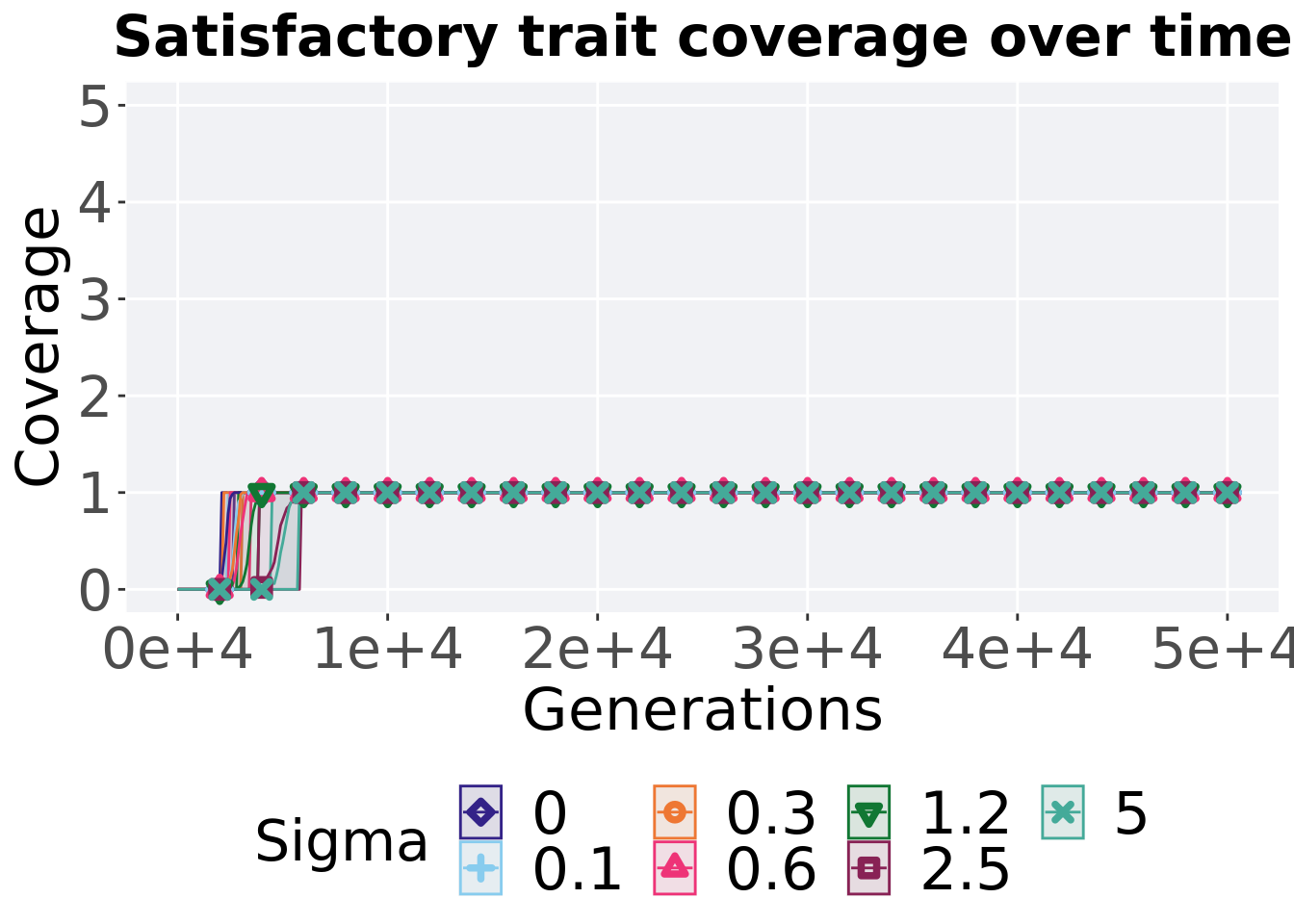

8.3.1.2 Best coverage throughout

Best satisfactory trait coverage throughout 50,000 generations.

filter(gfs_best, col == 'pop_uni_obj' & diagnostic == 'contradictory_objectives') %>%
  ggplot(., aes(x = Sigma, y = val, color = Sigma, fill = Sigma, shape = Sigma)) +
  geom_flat_violin(position = position_nudge(x = .2, y = 0), scale = 'width', alpha = 0.2) +
  geom_point(position = position_jitter(width = .1), size = 1.5, alpha = 1.0) +
  geom_boxplot(color = 'black', width = .2, outlier.shape = NA, alpha = 0.0) +
    scale_y_continuous(
      name="Coverage"
    ) +
      scale_x_discrete(
        name="Sigma"
      )+
  scale_shape_manual(values=SHAPE)+
  scale_colour_manual(values = cb_palette) +
  scale_fill_manual(values = cb_palette) +
  ggtitle("Best satisfactory trait coverage throughout")+
  p_theme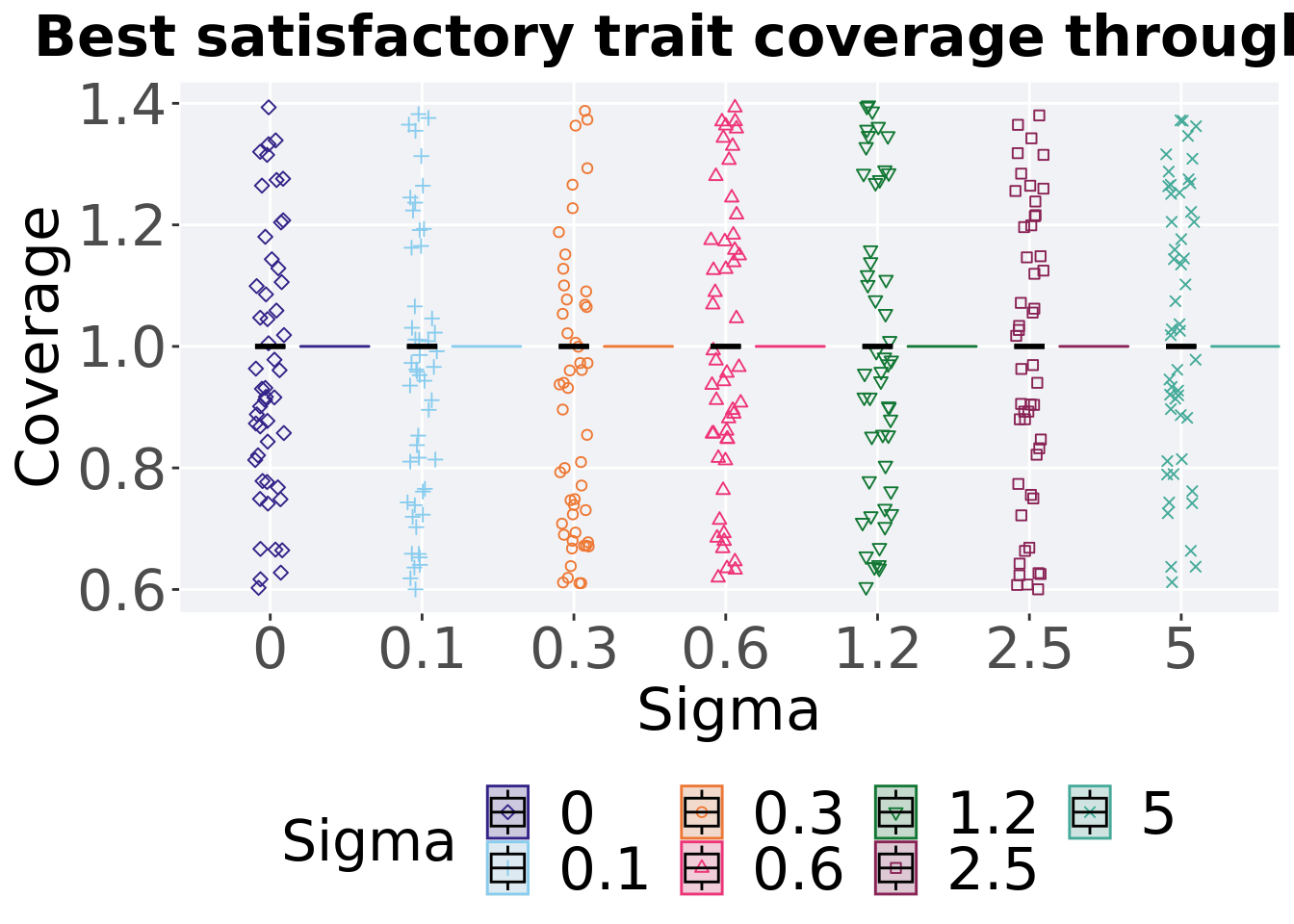

8.3.1.2.1 Stats

Summary statistics for the best satisfactory trait coverage throughout 50,000 generations.

coverage = filter(gfs_best, col == 'pop_uni_obj' & diagnostic == 'contradictory_objectives')
  group_by(coverage, Sigma) %>%
  dplyr::summarise(
    count = n(),
    na_cnt = sum(is.na(val)),
    min = min(val, na.rm = TRUE),
    median = median(val, na.rm = TRUE),
    mean = mean(val, na.rm = TRUE),
    max = max(val, na.rm = TRUE),
    IQR = IQR(val, na.rm = TRUE)
  )

## # A tibble: 7 x 8
##   Sigma count na_cnt   min median  mean   max   IQR
##   <fct> <int>  <int> <dbl>  <dbl> <dbl> <dbl> <dbl>
## 1 0        50      0     1      1     1     1     0
## 2 0.1      50      0     1      1     1     1     0
## 3 0.3      50      0     1      1     1     1     0
## 4 0.6      50      0     1      1     1     1     0
## 5 1.2      50      0     1      1     1     1     0
## 6 2.5      50      0     1      1     1     1     0
## 7 5        50      0     1      1     1     1     0

Kruskal–Wallis test provides evidence of no statistical difference among satisfactory trait coverage throughout 50,000 generations.

kruskal.test(val ~ Sigma, data = coverage)

## 
##  Kruskal-Wallis rank sum test
## 
## data:  val by Sigma
## Kruskal-Wallis chi-squared = NaN, df = 6, p-value = NA

8.3.1.3 End of 50,000 generations

Satisfactory trait coverage in the final population (50,000 generations).

filter(gfs_ot, diagnostic == 'contradictory_objectives' & gen == 50000) %>%
ggplot(., aes(x = Sigma, y = pop_uni_obj, color = Sigma, fill = Sigma, shape = Sigma)) +
  geom_flat_violin(position = position_nudge(x = .2, y = 0), scale = 'width', alpha = 0.2) +
  geom_point(position = position_jitter(width = .1), size = 1.5, alpha = 1.0) +
  geom_boxplot(color = 'black', width = .2, outlier.shape = NA, alpha = 0.0) +
  scale_y_continuous(
    name="Coverage",
    limits=c(0, 5)
  ) +
  scale_x_discrete(
    name="Sigma"
  )+
  scale_shape_manual(values=SHAPE)+
  scale_colour_manual(values = cb_palette) +
  scale_fill_manual(values = cb_palette) +
  ggtitle("Final satisfactory trait coverage") +
  p_theme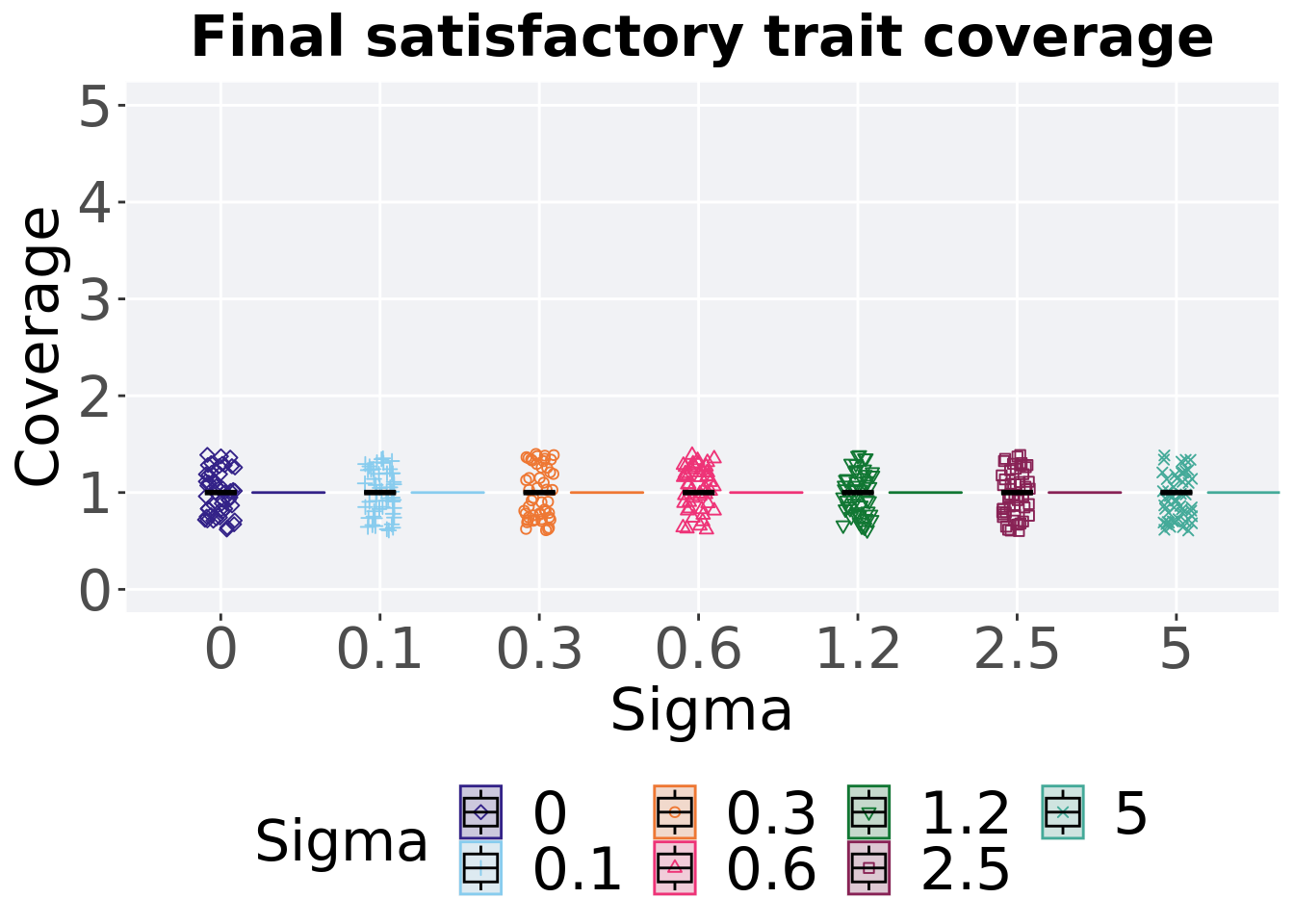

8.3.1.3.1 Stats

Summary statistics for satisfactory trait coverage in the final population (50,000 generations).

group_by(end, Sigma) %>%
  dplyr::summarise(
    count = n(),
    na_cnt = sum(is.na(pop_uni_obj)),
    min = min(pop_uni_obj, na.rm = TRUE),
    median = median(pop_uni_obj, na.rm = TRUE),
    mean = mean(pop_uni_obj, na.rm = TRUE),
    max = max(pop_uni_obj, na.rm = TRUE),
    IQR = IQR(pop_uni_obj, na.rm = TRUE)
  )

## # A tibble: 7 x 8
##   Sigma count na_cnt   min median  mean   max   IQR
##   <fct> <int>  <int> <int>  <dbl> <dbl> <int> <dbl>
## 1 0        50      0     0      0  0        0     0
## 2 0.1      50      0     0      0  0.1      1     0
## 3 0.3      50      0     0      0  0.02     1     0
## 4 0.6      50      0     0      0  0.06     1     0
## 5 1.2      50      0     0      0  0.42     2     1
## 6 2.5      50      0     0      1  1        2     0
## 7 5        50      0     0      1  1.12     2     0

Kruskal–Wallis test provides evidence of no statistical difference among satisfactory trait coverage throughout 50,000 generations.

kruskal.test(pop_uni_obj ~ Sigma, data = end)

## 
##  Kruskal-Wallis rank sum test
## 
## data:  pop_uni_obj by Sigma
## Kruskal-Wallis chi-squared = 228.29, df = 6, p-value < 2.2e-16

8.3.2 Activation gene coverage

Here we analyze the activation gene coverage for each parameter replicate on the contradictory objectives diagnostic.

8.3.2.1 Coverage over time

Activation gene coverage over time.

lines = filter(gfs_ot, diagnostic == 'contradictory_objectives') %>%
  group_by(Sigma, gen) %>%
  dplyr::summarise(
    min = min(uni_str_pos),
    mean = mean(uni_str_pos),
    max = max(uni_str_pos)
  )

## `summarise()` has grouped output by 'Sigma'. You can override using the
## `.groups` argument.

ggplot(lines, aes(x=gen, y=mean, group = Sigma, fill =Sigma, color = Sigma, shape = Sigma)) +
  geom_ribbon(aes(ymin = min, ymax = max), alpha = 0.1) +
  geom_line(size = 0.5) +
  geom_point(data = filter(lines, gen %% 2000 == 0 & gen != 0), size = 1.5, stroke = 2.0, alpha = 1.0) +
  scale_y_continuous(
    name="Coverage",
    limits=c(-1, 101),
    breaks=seq(0,100, 20),
    labels=c("0", "20", "40", "60", "80", "100")
  ) +
  scale_x_continuous(
    name="Generations",
    limits=c(0, 50000),
    breaks=c(0, 10000, 20000, 30000, 40000, 50000),
    labels=c("0e+4", "1e+4", "2e+4", "3e+4", "4e+4", "5e+4")

  ) +
  scale_shape_manual(values=SHAPE)+
  scale_colour_manual(values = cb_palette) +
  scale_fill_manual(values = cb_palette) +
  ggtitle("Activation gene coverage over time") +
  p_theme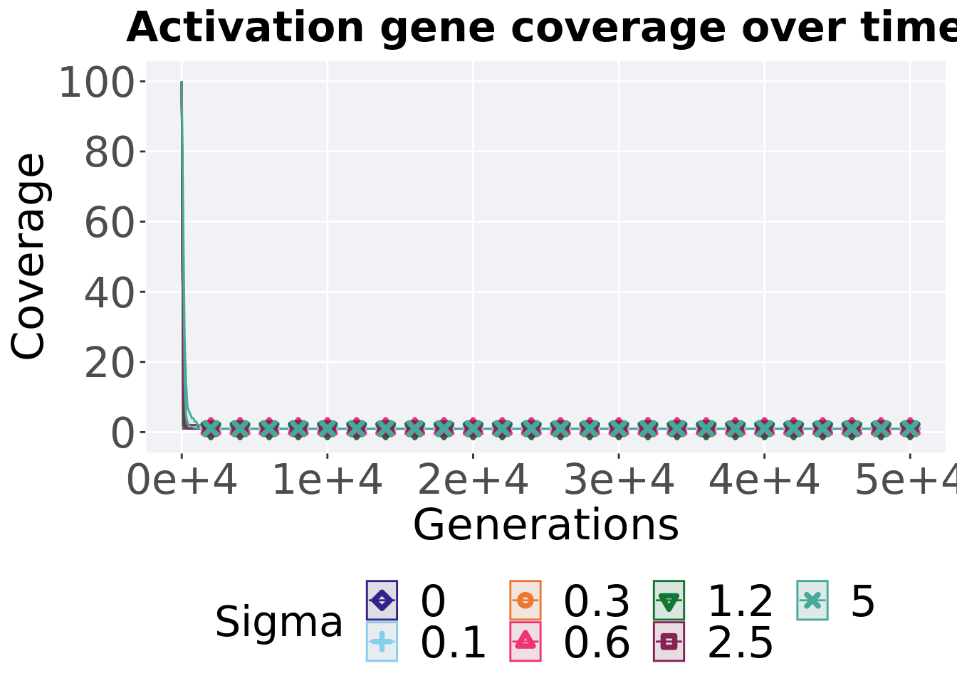

8.3.2.2 End of 50,000 generations

Activation gene coverage in the final population (50,000 generations).

filter(gfs_ot, diagnostic == 'contradictory_objectives' & gen == 50000) %>%
  ggplot(., aes(x = Sigma, y = uni_str_pos, color = Sigma, fill = Sigma, shape = Sigma)) +
    geom_flat_violin(position = position_nudge(x = .2, y = 0), scale = 'width', alpha = 0.2) +
    geom_point(position = position_jitter(width = .1), size = 1.5, alpha = 1.0) +
    geom_boxplot(color = 'black', width = .2, outlier.shape = NA, alpha = 0.0) +
    scale_y_continuous(
      name="Coverage",
      limits=c(0, 5)
    ) +
    scale_x_discrete(
      name="Sigma"
    )+
    scale_shape_manual(values=SHAPE)+
    scale_colour_manual(values = cb_palette) +
    scale_fill_manual(values = cb_palette) +
    ggtitle("Final activation gene coverage") +
    p_theme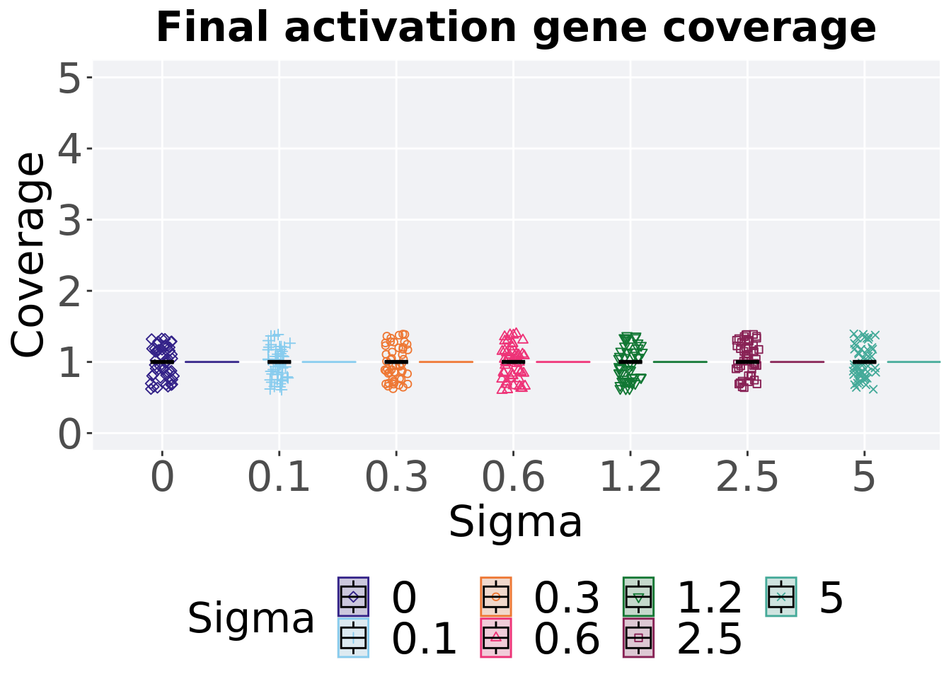

8.3.2.2.1 Stats

Summary statistics for activation gene coverage in the final population (50,000 generations).

coverage = filter(gfs_ot, diagnostic == 'contradictory_objectives' & gen == 50000)
group_by(coverage, Sigma) %>%
  dplyr::summarise(
    count = n(),
    na_cnt = sum(is.na(uni_str_pos)),
    min = min(uni_str_pos, na.rm = TRUE),
    median = median(uni_str_pos, na.rm = TRUE),
    mean = mean(uni_str_pos, na.rm = TRUE),
    max = max(uni_str_pos, na.rm = TRUE),
    IQR = IQR(uni_str_pos, na.rm = TRUE)
  )

## # A tibble: 7 x 8
##   Sigma count na_cnt   min median  mean   max   IQR
##   <fct> <int>  <int> <int>  <dbl> <dbl> <int> <dbl>
## 1 0        50      0     1      1     1     1     0
## 2 0.1      50      0     1      1     1     1     0
## 3 0.3      50      0     1      1     1     1     0
## 4 0.6      50      0     1      1     1     1     0
## 5 1.2      50      0     1      1     1     1     0
## 6 2.5      50      0     1      1     1     1     0
## 7 5        50      0     1      1     1     1     0

Kruskal–Wallis test provides evidence of no statistical difference for activation gene coverage in the final population (50,000 generations).

kruskal.test(uni_str_pos ~ Sigma,data = coverage)

## 
##  Kruskal-Wallis rank sum test
## 
## data:  uni_str_pos by Sigma
## Kruskal-Wallis chi-squared = NaN, df = 6, p-value = NA

8.3.3 Multi-valley crossing

8.3.3.1 Satisfactory trait coverage over time

lines = filter(gfs_ot_mvc, diagnostic == 'contradictory_objectives') %>%
  group_by(Sigma, gen) %>%
  dplyr::summarise(
    min = min(pop_uni_obj),
    mean = mean(pop_uni_obj),
    max = max(pop_uni_obj)
  )

## `summarise()` has grouped output by 'Sigma'. You can override using the
## `.groups` argument.

ggplot(lines, aes(x=gen, y=mean, group = Sigma, fill =Sigma, color = Sigma, shape = Sigma)) +
  geom_ribbon(aes(ymin = min, ymax = max), alpha = 0.1) +
  geom_line(size = 0.5) +
  geom_point(data = filter(lines, gen %% 2000 == 0 & gen != 0), size = 1.5, stroke = 2.0, alpha = 1.0) +
  scale_y_continuous(
    name="Coverage",
    limits=c(0, 5)
  ) +
  scale_x_continuous(
    name="Generations",
    limits=c(0, 50000),
    breaks=c(0, 10000, 20000, 30000, 40000, 50000),
    labels=c("0e+4", "1e+4", "2e+4", "3e+4", "4e+4", "5e+4")

  ) +
  scale_shape_manual(values=SHAPE)+
  scale_colour_manual(values = cb_palette) +
  scale_fill_manual(values = cb_palette) +
  ggtitle("Satisfactory trait coverage over time") +
  p_theme

8.3.3.2 Satisfactory trait coverage comparison

Best performances in the population at 40,000 and 50,000 generations.

# 80% and final generation comparison
end = filter(gfs_ot_mvc, diagnostic == 'contradictory_objectives' & gen == 50000)
end$Generation <- factor(end$gen)

mid = filter(gfs_ot_mvc, diagnostic == 'contradictory_objectives' & gen == 40000)
mid$Generation <- factor(mid$gen)

mvc_p = ggplot(mid, aes(x = Sigma, y=pop_uni_obj, group = Sigma, shape = Generation)) +
  geom_point(col = mvc_col[1] , position = position_jitternudge(jitter.width = .03, nudge.x = -0.05), size = 2, alpha = 1.0) +
  geom_boxplot(position = position_nudge(x = -.15, y = 0), lwd = 0.7, col = mvc_col[1], fill = mvc_col[1], width = .1, outlier.shape = NA, alpha = 0.0) +

  geom_point(data = end, aes(x = Sigma, y=pop_uni_obj), col = mvc_col[2], position = position_jitternudge(jitter.width = .03, nudge.x = 0.05), size = 2, alpha = 1.0) +
  geom_boxplot(data = end, aes(x = Sigma, y=pop_uni_obj), position = position_nudge(x = .15, y = 0), lwd = 0.7, col = mvc_col[2], fill = mvc_col[2], width = .1, outlier.shape = NA, alpha = 0.0) +

  scale_y_continuous(
    name="Coverage",
  ) +
  scale_x_discrete(
    name="Sigma"
  )+
  scale_shape_manual(values=c(0,1))+
  scale_colour_manual(values = c(mvc_col[1],mvc_col[2])) +
  p_theme

plot_grid(
  mvc_p +
    ggtitle("Satisfactory trait coverage over time") +
    theme(legend.position="none"),
  legend,
  nrow=2,
  rel_heights = c(1,.05),
  label_size = TSIZE
)

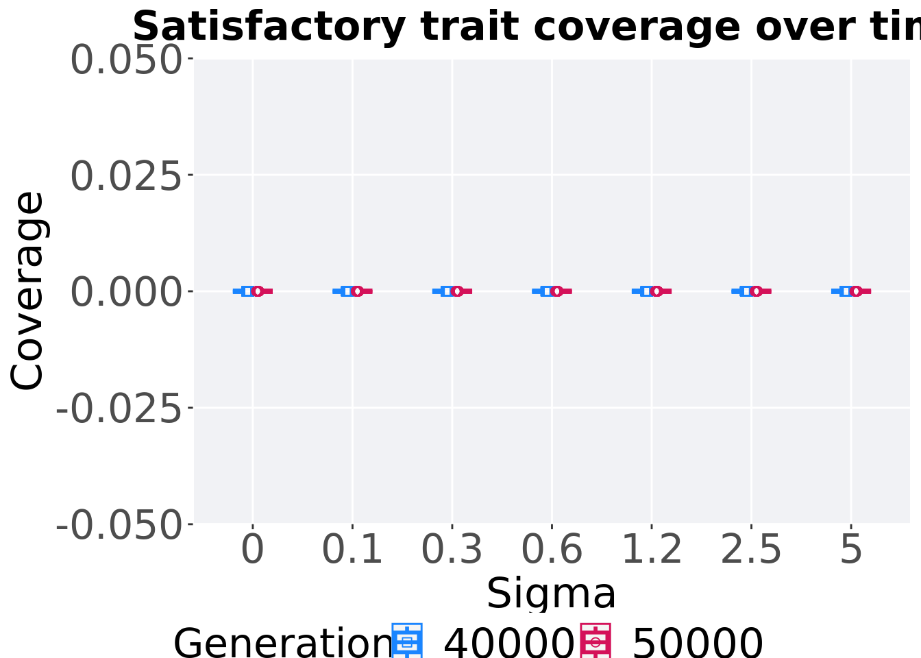
8.3.3.2.1 Stats

Summary statistics for the performance of the best performance at 40,000 and 50,000 generations.

slices = filter(gfs_ot_mvc, diagnostic == 'contradictory_objectives' & (gen == 50000 | gen == 40000))
slices$Generation <- factor(slices$gen, levels = c(50000,40000))
slices %>%
  group_by(Sigma, Generation) %>%
  dplyr::summarise(
    count = n(),
    na_cnt = sum(is.na(pop_uni_obj)),
    min = min(pop_uni_obj, na.rm = TRUE),
    median = median(pop_uni_obj, na.rm = TRUE),
    mean = mean(pop_uni_obj, na.rm = TRUE),
    max = max(pop_uni_obj, na.rm = TRUE),
    IQR = IQR(pop_uni_obj, na.rm = TRUE)
  )

## `summarise()` has grouped output by 'Sigma'. You can override using the
## `.groups` argument.

## # A tibble: 14 x 9
## # Groups:   Sigma [7]
##    Sigma Generation count na_cnt   min median  mean   max   IQR
##    <fct> <fct>      <int>  <int> <int>  <dbl> <dbl> <int> <dbl>
##  1 0     50000         50      0     0      0     0     0     0
##  2 0     40000         50      0     0      0     0     0     0
##  3 0.1   50000         50      0     0      0     0     0     0
##  4 0.1   40000         50      0     0      0     0     0     0
##  5 0.3   50000         50      0     0      0     0     0     0
##  6 0.3   40000         50      0     0      0     0     0     0
##  7 0.6   50000         50      0     0      0     0     0     0
##  8 0.6   40000         50      0     0      0     0     0     0
##  9 1.2   50000         50      0     0      0     0     0     0
## 10 1.2   40000         50      0     0      0     0     0     0
## 11 2.5   50000         50      0     0      0     0     0     0
## 12 2.5   40000         50      0     0      0     0     0     0
## 13 5     50000         50      0     0      0     0     0     0
## 14 5     40000         50      0     0      0     0     0     0

Sigma 0.0

wilcox.test(x = filter(slices, Sigma == 0.0 & Generation == 50000)$pop_uni_obj,
            y = filter(slices, Sigma == 0.0 & Generation == 40000)$pop_uni_obj,
            alternative = 't')

## 
##  Wilcoxon rank sum test with continuity correction
## 
## data:  filter(slices, Sigma == 0 & Generation == 50000)$pop_uni_obj and filter(slices, Sigma == 0 & Generation == 40000)$pop_uni_obj
## W = 1250, p-value = NA
## alternative hypothesis: true location shift is not equal to 0

Sigma 0.1

wilcox.test(x = filter(slices, Sigma == 0.1 & Generation == 50000)$pop_uni_obj,
            y = filter(slices, Sigma == 0.1 & Generation == 40000)$pop_uni_obj,
            alternative = 't')

## 
##  Wilcoxon rank sum test with continuity correction
## 
## data:  filter(slices, Sigma == 0.1 & Generation == 50000)$pop_uni_obj and filter(slices, Sigma == 0.1 & Generation == 40000)$pop_uni_obj
## W = 1250, p-value = NA
## alternative hypothesis: true location shift is not equal to 0

Sigma 0.3

wilcox.test(x = filter(slices, Sigma == 0.3 & Generation == 50000)$pop_uni_obj,
            y = filter(slices, Sigma == 0.3 & Generation == 40000)$pop_uni_obj,
            alternative = 't')

## 
##  Wilcoxon rank sum test with continuity correction
## 
## data:  filter(slices, Sigma == 0.3 & Generation == 50000)$pop_uni_obj and filter(slices, Sigma == 0.3 & Generation == 40000)$pop_uni_obj
## W = 1250, p-value = NA
## alternative hypothesis: true location shift is not equal to 0

Sigma 0.6

wilcox.test(x = filter(slices, Sigma == 0.6 & Generation == 50000)$pop_uni_obj,
            y = filter(slices, Sigma == 0.6 & Generation == 40000)$pop_uni_obj,
            alternative = 't')

## 
##  Wilcoxon rank sum test with continuity correction
## 
## data:  filter(slices, Sigma == 0.6 & Generation == 50000)$pop_uni_obj and filter(slices, Sigma == 0.6 & Generation == 40000)$pop_uni_obj
## W = 1250, p-value = NA
## alternative hypothesis: true location shift is not equal to 0

Sigma 1.2

wilcox.test(x = filter(slices, Sigma == 1.2 & Generation == 50000)$pop_uni_obj,
            y = filter(slices, Sigma == 1.2 & Generation == 40000)$pop_uni_obj,
            alternative = 't')

## 
##  Wilcoxon rank sum test with continuity correction
## 
## data:  filter(slices, Sigma == 1.2 & Generation == 50000)$pop_uni_obj and filter(slices, Sigma == 1.2 & Generation == 40000)$pop_uni_obj
## W = 1250, p-value = NA
## alternative hypothesis: true location shift is not equal to 0

Sigma 2.5

wilcox.test(x = filter(slices, Sigma == 2.5 & Generation == 50000)$pop_uni_obj,
            y = filter(slices, Sigma == 2.5 & Generation == 40000)$pop_uni_obj,
            alternative = 't')

## 
##  Wilcoxon rank sum test with continuity correction
## 
## data:  filter(slices, Sigma == 2.5 & Generation == 50000)$pop_uni_obj and filter(slices, Sigma == 2.5 & Generation == 40000)$pop_uni_obj
## W = 1250, p-value = NA
## alternative hypothesis: true location shift is not equal to 0

Sigma 5.0

wilcox.test(x = filter(slices, Sigma == 5.0 & Generation == 50000)$pop_uni_obj,
            y = filter(slices, Sigma == 5.0 & Generation == 40000)$pop_uni_obj,
            alternative = 't')

## 
##  Wilcoxon rank sum test with continuity correction
## 
## data:  filter(slices, Sigma == 5 & Generation == 50000)$pop_uni_obj and filter(slices, Sigma == 5 & Generation == 40000)$pop_uni_obj
## W = 1250, p-value = NA
## alternative hypothesis: true location shift is not equal to 0

8.3.3.3 Activation gene coverage over time

lines = filter(gfs_ot_mvc, diagnostic == 'contradictory_objectives') %>%
  group_by(Sigma, gen) %>%
  dplyr::summarise(
    min = min(uni_str_pos),
    mean = mean(uni_str_pos),
    max = max(uni_str_pos)
  )

## `summarise()` has grouped output by 'Sigma'. You can override using the
## `.groups` argument.

ggplot(lines, aes(x=gen, y=mean, group = Sigma, fill =Sigma, color = Sigma, shape = Sigma)) +
  geom_ribbon(aes(ymin = min, ymax = max), alpha = 0.1) +
  geom_line(size = 0.5) +
  geom_point(data = filter(lines, gen %% 2000 == 0 & gen != 0), size = 1.5, stroke = 2.0, alpha = 1.0) +
  scale_y_continuous(
    name="Coverage"
  ) +
  scale_x_continuous(
    name="Generations",
    limits=c(0, 50000),
    breaks=c(0, 10000, 20000, 30000, 40000, 50000),
    labels=c("0e+4", "1e+4", "2e+4", "3e+4", "4e+4", "5e+4")

  ) +
  scale_shape_manual(values=SHAPE)+
  scale_colour_manual(values = cb_palette) +
  scale_fill_manual(values = cb_palette) +
  ggtitle("Activation gene coverage over time") +
  p_theme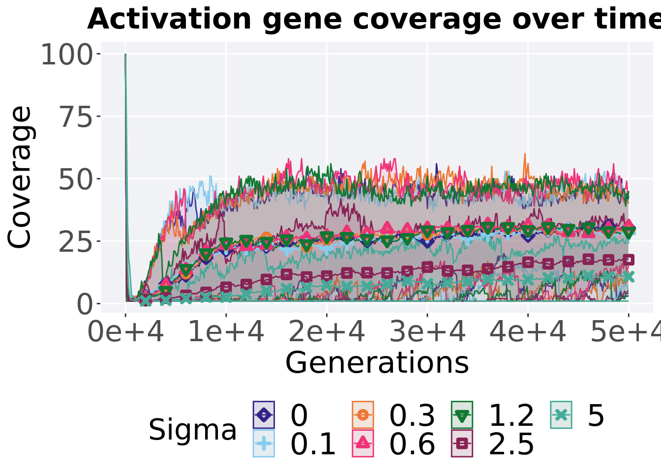

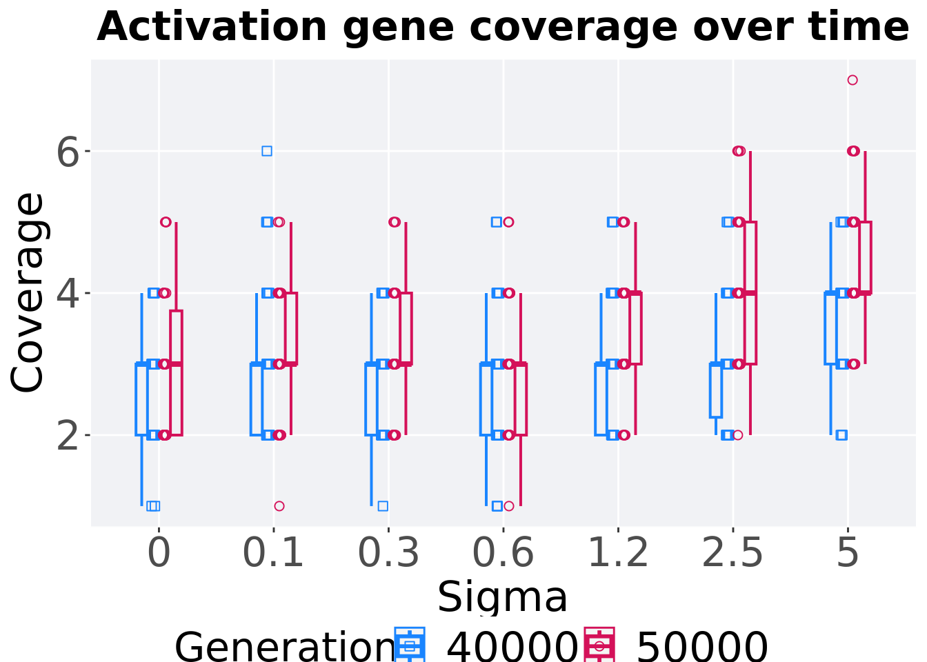
8.3.3.4 Activation gene coverage comparison

Activation gene coverage in the population at 40,000 and 50,000 generations.

# 80% and final generation comparison
end = filter(gfs_ot_mvc, diagnostic == 'contradictory_objectives' & gen == 50000)
end$Generation <- factor(end$gen)

mid = filter(gfs_ot_mvc, diagnostic == 'contradictory_objectives' & gen == 40000)
mid$Generation <- factor(mid$gen)

mvc_p = ggplot(mid, aes(x = Sigma, y=uni_str_pos, group = Sigma, shape = Generation)) +
  geom_point(col = mvc_col[1] , position = position_jitternudge(jitter.width = .03, nudge.x = -0.05), size = 2, alpha = 1.0) +
  geom_boxplot(position = position_nudge(x = -.15, y = 0), lwd = 0.7, col = mvc_col[1], fill = mvc_col[1], width = .1, outlier.shape = NA, alpha = 0.0) +

  geom_point(data = end, aes(x = Sigma, y=uni_str_pos), col = mvc_col[2], position = position_jitternudge(jitter.width = .03, nudge.x = 0.05), size = 2, alpha = 1.0) +
  geom_boxplot(data = end, aes(x = Sigma, y=uni_str_pos), position = position_nudge(x = .15, y = 0), lwd = 0.7, col = mvc_col[2], fill = mvc_col[2], width = .1, outlier.shape = NA, alpha = 0.0) +

  scale_y_continuous(
    name="Coverage",
  ) +
  scale_x_discrete(
    name="Sigma"
  )+
  scale_shape_manual(values=c(0,1))+
  scale_colour_manual(values = c(mvc_col[1],mvc_col[2])) +
  p_theme

plot_grid(
  mvc_p +
    ggtitle("Satisfactory trait coverage over time") +
    theme(legend.position="none"),
  legend,
  nrow=2,
  rel_heights = c(1,.05),
  label_size = TSIZE
)

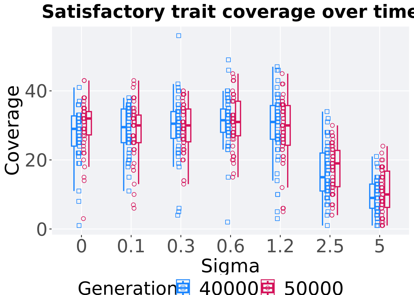
8.3.3.4.1 Stats

Summary statistics for the activation gene coverage at 40,000 and 50,000 generations.

slices = filter(gfs_ot_mvc, diagnostic == 'contradictory_objectives' & (gen == 50000 | gen == 40000))
slices$Generation <- factor(slices$gen, levels = c(50000,40000))
slices %>%
  group_by(Sigma, Generation) %>%
  dplyr::summarise(
    count = n(),
    na_cnt = sum(is.na(uni_str_pos)),
    min = min(uni_str_pos, na.rm = TRUE),
    median = median(uni_str_pos, na.rm = TRUE),
    mean = mean(uni_str_pos, na.rm = TRUE),
    max = max(uni_str_pos, na.rm = TRUE),
    IQR = IQR(uni_str_pos, na.rm = TRUE)
  )

## `summarise()` has grouped output by 'Sigma'. You can override using the
## `.groups` argument.

## # A tibble: 14 x 9
## # Groups:   Sigma [7]
##    Sigma Generation count na_cnt   min median  mean   max   IQR
##    <fct> <fct>      <int>  <int> <int>  <dbl> <dbl> <int> <dbl>
##  1 0     50000         50      0     3   32    30.2    43  6.75
##  2 0     40000         50      0     1   29    27.3    41  8.75
##  3 0.1   50000         50      0     6   30    28.1    43  8   
##  4 0.1   40000         50      0    11   29.5  28.7    38  9.75
##  5 0.3   50000         50      0    13   30    29.4    40  9.5 
##  6 0.3   40000         50      0     4   30.5  29.3    56  7.75
##  7 0.6   50000         50      0    15   31    30.8    45 10   
##  8 0.6   40000         50      0     2   31.5  31.2    49  6.75
##  9 1.2   50000         50      0     5   30    28.8    45 11.5 
## 10 1.2   40000         50      0     3   31    29.4    47  9.75
## 11 2.5   50000         50      0     4   19    17.5    30 10.5 
## 12 2.5   40000         50      0     1   15    16.5    34 11   
## 13 5     50000         50      0     1   10    10.8    24 10.5 
## 14 5     40000         50      0     1    9     9.5    21  7

Sigma 0.0

wilcox.test(x = filter(slices, Sigma == 0.0 & Generation == 50000)$uni_str_pos,
            y = filter(slices, Sigma == 0.0 & Generation == 40000)$uni_str_pos,
            alternative = 't')

## 
##  Wilcoxon rank sum test with continuity correction
## 
## data:  filter(slices, Sigma == 0 & Generation == 50000)$uni_str_pos and filter(slices, Sigma == 0 & Generation == 40000)$uni_str_pos
## W = 1599, p-value = 0.01605
## alternative hypothesis: true location shift is not equal to 0

Sigma 0.1

wilcox.test(x = filter(slices, Sigma == 0.1 & Generation == 50000)$uni_str_pos,
            y = filter(slices, Sigma == 0.1 & Generation == 40000)$uni_str_pos,
            alternative = 't')

## 
##  Wilcoxon rank sum test with continuity correction
## 
## data:  filter(slices, Sigma == 0.1 & Generation == 50000)$uni_str_pos and filter(slices, Sigma == 0.1 & Generation == 40000)$uni_str_pos
## W = 1211, p-value = 0.7903
## alternative hypothesis: true location shift is not equal to 0

Sigma 0.3

wilcox.test(x = filter(slices, Sigma == 0.3 & Generation == 50000)$uni_str_pos,
            y = filter(slices, Sigma == 0.3 & Generation == 40000)$uni_str_pos,
            alternative = 't')

## 
##  Wilcoxon rank sum test with continuity correction
## 
## data:  filter(slices, Sigma == 0.3 & Generation == 50000)$uni_str_pos and filter(slices, Sigma == 0.3 & Generation == 40000)$uni_str_pos
## W = 1223.5, p-value = 0.8575
## alternative hypothesis: true location shift is not equal to 0

Sigma 0.6

wilcox.test(x = filter(slices, Sigma == 0.6 & Generation == 50000)$uni_str_pos,
            y = filter(slices, Sigma == 0.6 & Generation == 40000)$uni_str_pos,
            alternative = 't')

## 
##  Wilcoxon rank sum test with continuity correction
## 
## data:  filter(slices, Sigma == 0.6 & Generation == 50000)$uni_str_pos and filter(slices, Sigma == 0.6 & Generation == 40000)$uni_str_pos
## W = 1163, p-value = 0.5502
## alternative hypothesis: true location shift is not equal to 0

Sigma 1.2

wilcox.test(x = filter(slices, Sigma == 1.2 & Generation == 50000)$uni_str_pos,
            y = filter(slices, Sigma == 1.2 & Generation == 40000)$uni_str_pos,
            alternative = 't')

## 
##  Wilcoxon rank sum test with continuity correction
## 
## data:  filter(slices, Sigma == 1.2 & Generation == 50000)$uni_str_pos and filter(slices, Sigma == 1.2 & Generation == 40000)$uni_str_pos
## W = 1194, p-value = 0.7017
## alternative hypothesis: true location shift is not equal to 0

Sigma 2.5

wilcox.test(x = filter(slices, Sigma == 2.5 & Generation == 50000)$uni_str_pos,
            y = filter(slices, Sigma == 2.5 & Generation == 40000)$uni_str_pos,
            alternative = 't')

## 
##  Wilcoxon rank sum test with continuity correction
## 
## data:  filter(slices, Sigma == 2.5 & Generation == 50000)$uni_str_pos and filter(slices, Sigma == 2.5 & Generation == 40000)$uni_str_pos
## W = 1380.5, p-value = 0.3696
## alternative hypothesis: true location shift is not equal to 0

Sigma 5.0

wilcox.test(x = filter(slices, Sigma == 5.0 & Generation == 50000)$uni_str_pos,
            y = filter(slices, Sigma == 5.0 & Generation == 40000)$uni_str_pos,
            alternative = 't')

## 
##  Wilcoxon rank sum test with continuity correction
## 
## data:  filter(slices, Sigma == 5 & Generation == 50000)$uni_str_pos and filter(slices, Sigma == 5 & Generation == 40000)$uni_str_pos
## W = 1381.5, p-value = 0.3656
## alternative hypothesis: true location shift is not equal to 0

8.4 Multi-path exploration results

Here we present the results for best performances and activation gene coverage found by each genotypic fitness sharing sigma value replicate on the multi-path exploration diagnostic. Best performance found refers to the largest average trait score found in a given population, while activation gene coverage refers to the count of unique activation genes in the population. Note that both values fall between 0 and 100.

8.4.1 Performance

Here we analyze the performances for each parameter replicate on the multi-path exploration diagnostic.

8.4.1.1 Performance over time

Performance over time.

lines = filter(gfs_ot, diagnostic == 'multipath_exploration') %>%
  group_by(Sigma, gen) %>%
  dplyr::summarise(
    min = min(pop_fit_max),
    mean = mean(pop_fit_max),
    max = max(pop_fit_max)
  )

## `summarise()` has grouped output by 'Sigma'. You can override using the
## `.groups` argument.

ggplot(lines, aes(x=gen, y=mean / DIMENSIONALITY, group = Sigma, fill = Sigma, color = Sigma, shape = Sigma)) +
  geom_ribbon(aes(ymin = min / DIMENSIONALITY, ymax = max / DIMENSIONALITY), alpha = 0.1) +
  geom_line(size = 0.5) +
  geom_point(data = filter(lines, gen %% 2000 == 0 & gen != 0), size = 1.5, stroke = 2.0, alpha = 1.0) +
  scale_y_continuous(
    name="Average trait score",
    limits=c(-1, 30)
  ) +
  scale_x_continuous(
    name="Generations",
    limits=c(0, 50000),
    breaks=c(0, 10000, 20000, 30000, 40000, 50000),
    labels=c("0e+4", "1e+4", "2e+4", "3e+4", "4e+4", "5e+4")

  ) +
  scale_shape_manual(values=SHAPE)+
  scale_colour_manual(values = cb_palette) +
  scale_fill_manual(values = cb_palette) +
  ggtitle("Best performance over time") +
  p_theme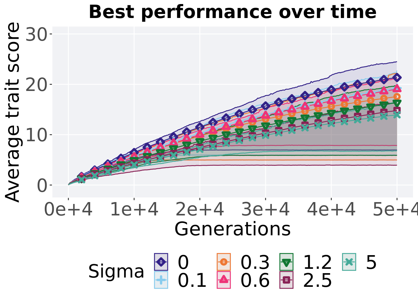

8.4.1.2 Best performance throughout

Here we plot the performance of the best performing solution found throughout 50,000 generations.

filter(gfs_best, col == 'pop_fit_max' & diagnostic == 'multipath_exploration') %>%
  ggplot(., aes(x = Sigma, y = val / DIMENSIONALITY, color = Sigma, fill = Sigma, shape = Sigma)) +
  geom_flat_violin(position = position_nudge(x = .2, y = 0), scale = 'width', alpha = 0.2) +
  geom_point(position = position_jitter(width = .1), size = 1.5, alpha = 1.0) +
  geom_boxplot(color = 'black', width = .2, outlier.shape = NA, alpha = 0.0) +
  scale_y_continuous(
    name="Average trait score",
    limits=c(-1, 30)
  ) +
  scale_x_discrete(
    name="Sigma"
  )+
  scale_shape_manual(values=SHAPE)+
  scale_colour_manual(values = cb_palette) +
  scale_fill_manual(values = cb_palette) +
  ggtitle("Best performance throughout") +
  p_theme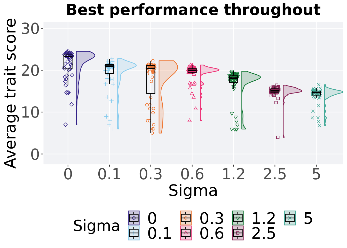

8.4.1.2.1 Stats

Summary statistics for the performance of the best performing solution.

performance = filter(gfs_best, col == 'pop_fit_max' & diagnostic == 'multipath_exploration')
group_by(performance, Sigma) %>%
dplyr::summarise(
  count = n(),
  na_cnt = sum(is.na(val)),
  min = min(val / DIMENSIONALITY, na.rm = TRUE),
  median = median(val / DIMENSIONALITY, na.rm = TRUE),
  mean = mean(val / DIMENSIONALITY, na.rm = TRUE),
  max = max(val / DIMENSIONALITY, na.rm = TRUE),
  IQR = IQR(val / DIMENSIONALITY, na.rm = TRUE)
)

## # A tibble: 7 x 8
##   Sigma count na_cnt   min median  mean   max   IQR
##   <fct> <int>  <int> <dbl>  <dbl> <dbl> <dbl> <dbl>
## 1 0        50      0  6.99   23.2  21.4  24.5 3.34 
## 2 0.1      50      0  5.98   21.0  19.3  22.7 2.12 
## 3 0.3      50      0  4.99   20.4  17.6  22.2 6.69 
## 4 0.6      50      0  7.93   20.0  19.1  21.2 0.841
## 5 1.2      50      0  5.95   18.1  16.4  19.8 1.55 
## 6 2.5      50      0  3.99   15.1  14.9  16.4 0.809
## 7 5        50      0  6.81   14.6  14.0  16.5 0.962

Kruskal–Wallis test provides evidence of statistical differences among the best performing solution.

kruskal.test(val ~ Sigma,data = performance)

## 
##  Kruskal-Wallis rank sum test
## 
## data:  val by Sigma
## Kruskal-Wallis chi-squared = 161.29, df = 6, p-value < 2.2e-16

Results for post-hoc Wilcoxon rank-sum test with a Bonferroni correction on the best performing solution.

pairwise.wilcox.test(x = performance$val, g = performance$Sigma , p.adjust.method = "bonferroni",
                     paired = FALSE, conf.int = FALSE, alternative = 'l')

## 
##  Pairwise comparisons using Wilcoxon rank sum test with continuity correction 
## 
## data:  performance$val and performance$Sigma 
## 
##     0       0.1     0.3     0.6     1.2     2.5    
## 0.1 0.00026 -       -       -       -       -      
## 0.3 4.8e-06 0.53186 -       -       -       -      
## 0.6 8.5e-06 0.00531 1.00000 -       -       -      
## 1.2 8.7e-09 2.1e-07 0.00023 2.7e-08 -       -      
## 2.5 1.0e-11 4.1e-10 0.00024 4.2e-12 6.6e-08 -      
## 5   9.4e-13 2.2e-10 9.9e-05 8.9e-13 3.7e-08 0.00268
## 
## P value adjustment method: bonferroni

8.4.1.3 End of 50,000 generations

Best performance in the final population (50,000 generations).

filter(gfs_ot, diagnostic == 'multipath_exploration' & gen == 50000) %>%
ggplot(., aes(x = Sigma, y = pop_fit_max / DIMENSIONALITY, color = Sigma, fill = Sigma, shape = Sigma)) +
  geom_flat_violin(position = position_nudge(x = .2, y = 0), scale = 'width', alpha = 0.2) +
  geom_point(position = position_jitter(width = .1), size = 1.5, alpha = 1.0) +
  geom_boxplot(color = 'black', width = .2, outlier.shape = NA, alpha = 0.0) +
  scale_y_continuous(
    name="Average trait score",
    limits=c(-1, 30)
  ) +
  scale_x_discrete(
    name="Sigma"
  )+
  scale_shape_manual(values=SHAPE)+
  scale_colour_manual(values = cb_palette) +
  scale_fill_manual(values = cb_palette) +
  ggtitle("Final best performance") +
  p_theme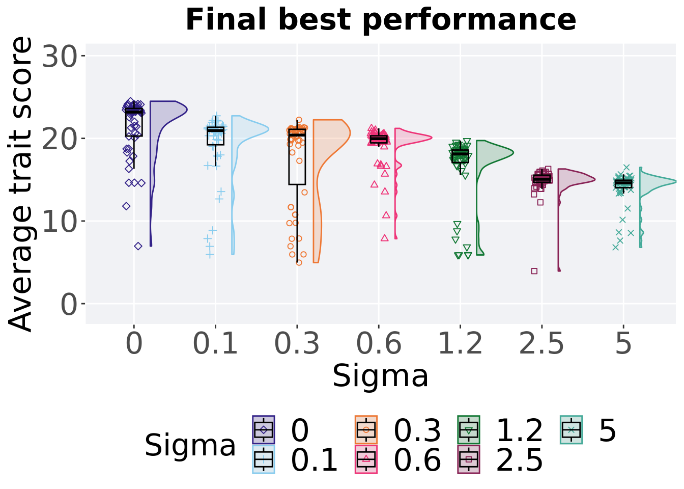

8.4.1.3.1 Stats

Summary statistics for the best performance in the final population (50,000 generations).

performance = filter(gfs_ot, diagnostic == 'multipath_exploration' & gen == 50000)
group_by(performance, Sigma) %>%
dplyr::summarise(
  count = n(),
  na_cnt = sum(is.na(pop_fit_max / DIMENSIONALITY)),
  min = min(pop_fit_max / DIMENSIONALITY, na.rm = TRUE),
  median = median(pop_fit_max / DIMENSIONALITY, na.rm = TRUE),
  mean = mean(pop_fit_max / DIMENSIONALITY, na.rm = TRUE),
  max = max(pop_fit_max / DIMENSIONALITY, na.rm = TRUE),
  IQR = IQR(pop_fit_max / DIMENSIONALITY, na.rm = TRUE)
)

## # A tibble: 7 x 8
##   Sigma count na_cnt   min median  mean   max   IQR
##   <fct> <int>  <int> <dbl>  <dbl> <dbl> <dbl> <dbl>
## 1 0        50      0  6.96   23.2  21.3  24.5 3.34 
## 2 0.1      50      0  5.95   20.9  19.3  22.7 2.12 
## 3 0.3      50      0  4.96   20.4  17.6  22.2 6.68 
## 4 0.6      50      0  7.85   20.0  19.0  21.2 0.855
## 5 1.2      50      0  5.89   18.1  16.3  19.7 1.51 
## 6 2.5      50      0  3.94   15.1  14.8  16.3 0.864
## 7 5        50      0  6.81   14.6  14.0  16.5 0.904

Kruskal–Wallis test provides evidence of statistical differences among best performance in the final population (50,000 generations).

kruskal.test(pop_fit_max ~ Sigma, data = performance)

## 
##  Kruskal-Wallis rank sum test
## 
## data:  pop_fit_max by Sigma
## Kruskal-Wallis chi-squared = 161.62, df = 6, p-value < 2.2e-16

Results for post-hoc Wilcoxon rank-sum test with a Bonferroni correction on the best performance in the final population (50,000 generations).

pairwise.wilcox.test(x = performance$pop_fit_max, g = performance$Sigma , p.adjust.method = "bonferroni",
                     paired = FALSE, conf.int = FALSE, alternative = 'l')

## 
##  Pairwise comparisons using Wilcoxon rank sum test with continuity correction 
## 
## data:  performance$pop_fit_max and performance$Sigma 
## 
##     0       0.1     0.3     0.6     1.2     2.5    
## 0.1 0.00024 -       -       -       -       -      
## 0.3 5.0e-06 0.45941 -       -       -       -      
## 0.6 8.2e-06 0.00431 1.00000 -       -       -      
## 1.2 6.7e-09 1.9e-07 0.00022 2.9e-08 -       -      
## 2.5 9.4e-12 4.1e-10 0.00024 4.4e-12 6.6e-08 -      
## 5   9.9e-13 2.2e-10 9.6e-05 8.9e-13 3.6e-08 0.00283
## 
## P value adjustment method: bonferroni

8.4.2 Activation gene coverage

Here we analyze the activation gene coverage for each parameter replicate on the multi-path exploration diagnostic.

8.4.2.1 Coverage over time

Activation gene coverage over time.

lines = filter(gfs_ot, diagnostic == 'multipath_exploration') %>%
  group_by(Sigma, gen) %>%
  dplyr::summarise(
    min = min(uni_str_pos),
    mean = mean(uni_str_pos),
    max = max(uni_str_pos)
  )

## `summarise()` has grouped output by 'Sigma'. You can override using the
## `.groups` argument.

ggplot(lines, aes(x=gen, y=mean, group = Sigma, fill =Sigma, color = Sigma, shape = Sigma)) +
  geom_ribbon(aes(ymin = min, ymax = max), alpha = 0.1) +
  geom_line(size = 0.5) +
  geom_point(data = filter(lines, gen %% 2000 == 0 & gen != 0), size = 1.5, stroke = 2.0, alpha = 1.0) +
  scale_y_continuous(
    name="Coverage",
    limits=c(-1, 101),
    breaks=seq(0,100, 20),
    labels=c("0", "20", "40", "60", "80", "100")
  ) +
  scale_x_continuous(
    name="Generations",
    limits=c(0, 50000),
    breaks=c(0, 10000, 20000, 30000, 40000, 50000),
    labels=c("0e+4", "1e+4", "2e+4", "3e+4", "4e+4", "5e+4")

  ) +
  scale_shape_manual(values=SHAPE)+
  scale_colour_manual(values = cb_palette) +
  scale_fill_manual(values = cb_palette) +
  ggtitle("Activation gene coverage over time") +
  p_theme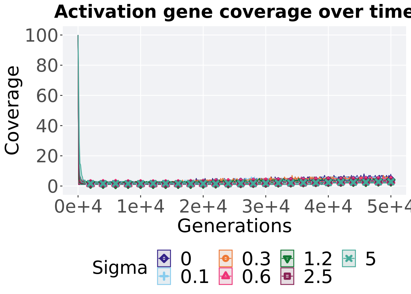

8.4.2.2 End of 50,000 generations

Activation gene coverage in the final population (50,000 generations).

filter(gfs_ot, diagnostic == 'multipath_exploration' & gen == 50000)%>%
ggplot(., aes(x = Sigma, y = uni_str_pos, color = Sigma, fill = Sigma, shape = Sigma)) +
  geom_flat_violin(position = position_nudge(x = .2, y = 0), scale = 'width', alpha = 0.2) +
  geom_point(position = position_jitter(width = .1), size = 1.5, alpha = 1.0) +
  geom_boxplot(color = 'black', width = .2, outlier.shape = NA, alpha = 0.0) +
  scale_y_continuous(
    name="Coverage",
    limits=c(-1, 10),
    breaks=seq(0,10, 2),
    labels=c("0", "2", "4", "6", "8", "10")
  ) +
  scale_x_discrete(
    name="Sigma"
  )+
  scale_shape_manual(values=SHAPE)+
  scale_colour_manual(values = cb_palette) +
  scale_fill_manual(values = cb_palette) +
  ggtitle("Final activation gene coverage") +
  p_theme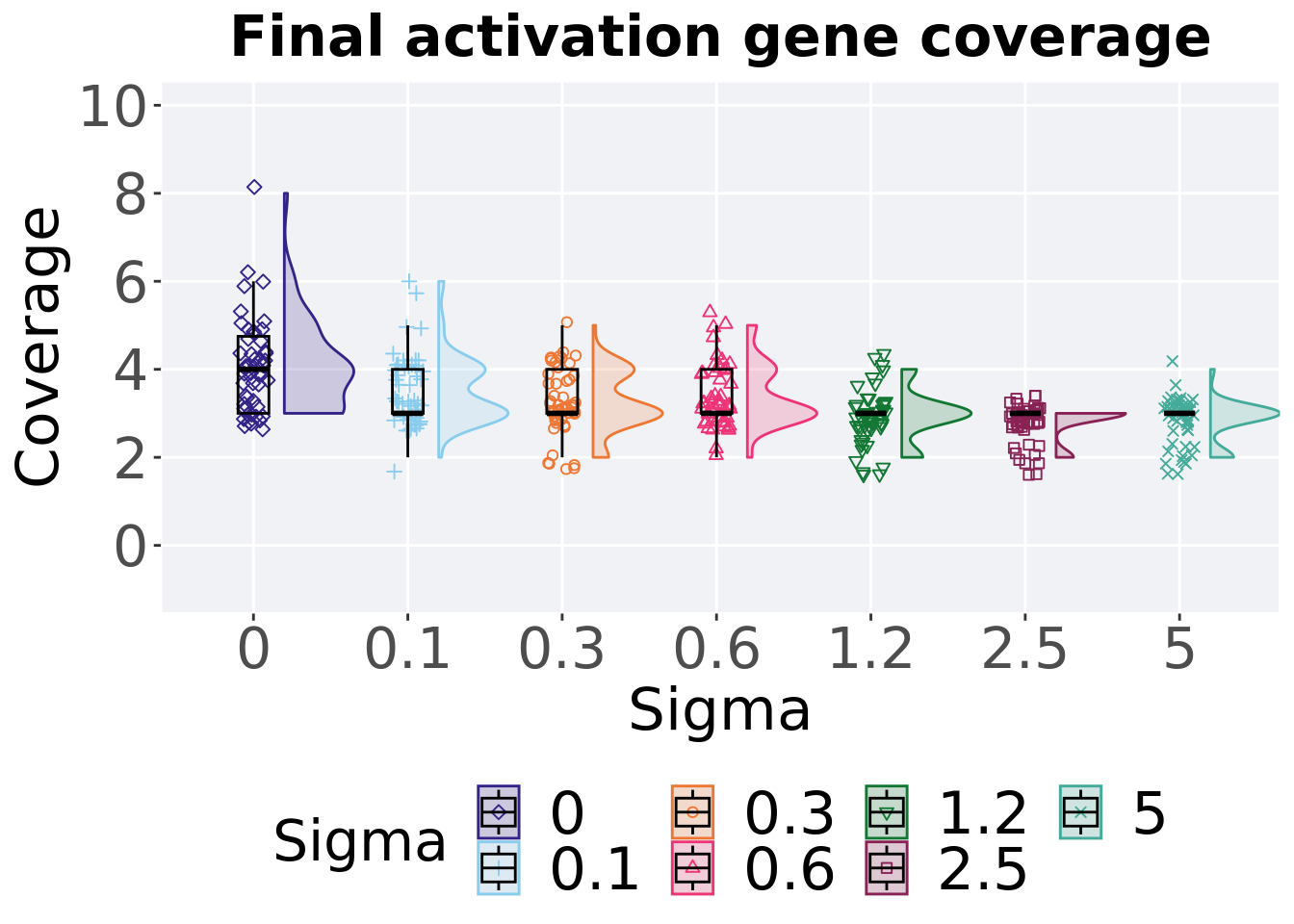

8.4.2.2.1 Stats

Summary statistics for the activation gene coverage in the final population (50,000 generations).

performance = filter(gfs_ot, diagnostic == 'multipath_exploration' & gen == 50000)
group_by(performance, Sigma) %>%
dplyr::summarise(
  count = n(),
  na_cnt = sum(is.na(uni_str_pos)),
  min = min(uni_str_pos, na.rm = TRUE),
  median = median(uni_str_pos, na.rm = TRUE),
  mean = mean(uni_str_pos, na.rm = TRUE),
  max = max(uni_str_pos, na.rm = TRUE),
  IQR = IQR(uni_str_pos, na.rm = TRUE)
)

## # A tibble: 7 x 8
##   Sigma count na_cnt   min median  mean   max   IQR
##   <fct> <int>  <int> <int>  <dbl> <dbl> <int> <dbl>
## 1 0        50      0     3      4  4.04     8  1.75
## 2 0.1      50      0     2      3  3.54     6  1   
## 3 0.3      50      0     2      3  3.24     5  1   
## 4 0.6      50      0     2      3  3.38     5  1   
## 5 1.2      50      0     2      3  2.94     4  0   
## 6 2.5      50      0     2      3  2.8      3  0   
## 7 5        50      0     2      3  2.8      4  0

Kruskal–Wallis test provides evidence of statistical differences among activation gene coverage in the final population (50,000 generations).

kruskal.test(uni_str_pos ~ Sigma, data = performance)

## 
##  Kruskal-Wallis rank sum test
## 
## data:  uni_str_pos by Sigma
## Kruskal-Wallis chi-squared = 93.885, df = 6, p-value < 2.2e-16

Results for post-hoc Wilcoxon rank-sum test with a Bonferroni correction on the activation gene coverage in the final population (50,000 generations).

pairwise.wilcox.test(x = performance$uni_str_pos, g = performance$Sigma , p.adjust.method = "bonferroni",
                     paired = FALSE, conf.int = FALSE, alternative = 't')

## 
##  Pairwise comparisons using Wilcoxon rank sum test with continuity correction 
## 
## data:  performance$uni_str_pos and performance$Sigma 
## 
##     0       0.1     0.3     0.6     1.2     2.5    
## 0.1 0.16972 -       -       -       -       -      
## 0.3 0.00109 1.00000 -       -       -       -      
## 0.6 0.00962 1.00000 1.00000 -       -       -      
## 1.2 1.2e-07 0.00138 0.48268 0.03870 -       -      
## 2.5 5.9e-11 7.7e-07 0.00563 6.8e-05 1.00000 -      
## 5   4.4e-10 4.4e-06 0.01196 0.00025 1.00000 1.00000
## 
## P value adjustment method: bonferroni

8.4.3 Multi-valley crossing

8.4.3.1 Performance over time

lines =  filter(gfs_ot_mvc, diagnostic == 'multipath_exploration') %>%
  group_by(Sigma, gen) %>%
  dplyr::summarise(
    min = min(pop_fit_max),
    mean = mean(pop_fit_max),
    max = max(pop_fit_max)
  )

## `summarise()` has grouped output by 'Sigma'. You can override using the
## `.groups` argument.

ggplot(lines, aes(x=gen, y=mean / DIMENSIONALITY, group = Sigma, fill = Sigma, color = Sigma, shape = Sigma)) +
  geom_ribbon(aes(ymin = min / DIMENSIONALITY, ymax = max / DIMENSIONALITY), alpha = 0.1) +
  geom_line(size = 0.5) +
  geom_point(data = filter(lines, gen %% 2000 == 0 & gen != 0), size = 1.5, stroke = 2.0, alpha = 1.0) +
  scale_y_continuous(
    name="Average trait score"
  ) +
  scale_x_continuous(
    name="Generations",
    limits=c(0, 50000),
    breaks=c(0, 10000, 20000, 30000, 40000, 50000),
    labels=c("0e+4", "1e+4", "2e+4", "3e+4", "4e+4", "5e+4")

  ) +
  scale_shape_manual(values=SHAPE)+
  scale_colour_manual(values = cb_palette) +
  scale_fill_manual(values = cb_palette) +
  ggtitle("Best performance over time") +
  p_theme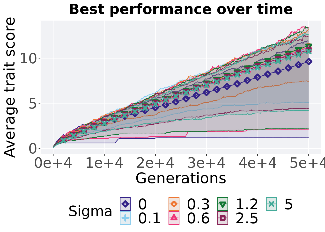

8.4.3.2 Performance comparisons

# 80% and final generation comparison
end = filter(gfs_ot_mvc, diagnostic == 'multipath_exploration' & gen == 50000)
end$Generation <- factor(end$gen)

mid = filter(gfs_ot_mvc, diagnostic == 'multipath_exploration' & gen == 40000)
mid$Generation <- factor(mid$gen)

mvc_p = ggplot(mid, aes(x = Sigma, y=pop_fit_max / DIMENSIONALITY, group = Sigma, shape = Generation)) +
  geom_point(col = mvc_col[1] , position = position_jitternudge(jitter.width = .03, nudge.x = -0.05), size = 2, alpha = 1.0) +
  geom_boxplot(position = position_nudge(x = -.15, y = 0), lwd = 0.7, col = mvc_col[1], fill = mvc_col[1], width = .1, outlier.shape = NA, alpha = 0.0) +

  geom_point(data = end, aes(x = Sigma, y=pop_fit_max / DIMENSIONALITY), col = mvc_col[2], position = position_jitternudge(jitter.width = .03, nudge.x = 0.05), size = 2, alpha = 1.0) +
  geom_boxplot(data = end, aes(x = Sigma, y=pop_fit_max / DIMENSIONALITY), position = position_nudge(x = .15, y = 0), lwd = 0.7, col = mvc_col[2], fill = mvc_col[2], width = .1, outlier.shape = NA, alpha = 0.0) +

  scale_y_continuous(
    name="Average trait score"
  ) +
  scale_x_discrete(
    name="Sigma"
  )+
  scale_shape_manual(values=c(0,1))+
  scale_colour_manual(values = c(mvc_col[1],mvc_col[2])) +
  p_theme

plot_grid(
  mvc_p +
    ggtitle("Performance comparisons") +
    theme(legend.position="none"),
  legend,
  nrow=2,
  rel_heights = c(1,.05),
  label_size = TSIZE
)

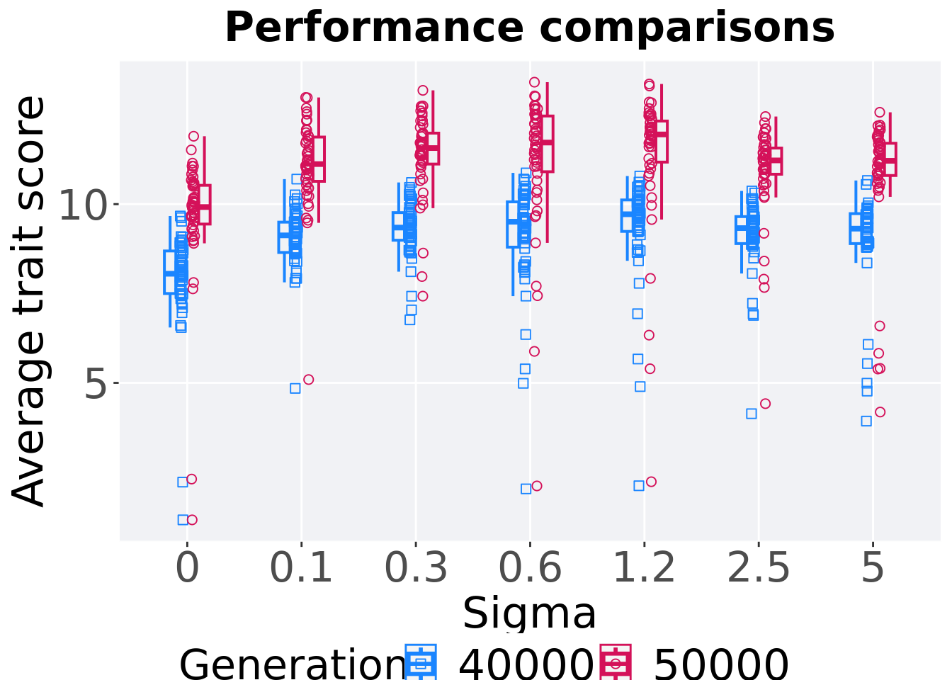
8.4.3.2.1 Stats

Summary statistics for the performance of the best performance at 40,000 and 50,000 generations.

# 80% and final generation comparison
slices = filter(gfs_ot_mvc, diagnostic == 'multipath_exploration' & (gen == 50000 | gen == 40000))
slices$Generation <- factor(slices$gen, levels = c(50000,40000))
slices %>%
  group_by(Sigma, Generation) %>%
  dplyr::summarise(
    count = n(),
    na_cnt = sum(is.na(pop_fit_max  / DIMENSIONALITY)),
    min = min(pop_fit_max  / DIMENSIONALITY, na.rm = TRUE),
    median = median(pop_fit_max  / DIMENSIONALITY, na.rm = TRUE),
    mean = mean(pop_fit_max  / DIMENSIONALITY, na.rm = TRUE),
    max = max(pop_fit_max  / DIMENSIONALITY, na.rm = TRUE),
    IQR = IQR(pop_fit_max  / DIMENSIONALITY, na.rm = TRUE)
  )

## `summarise()` has grouped output by 'Sigma'. You can override using the
## `.groups` argument.

## # A tibble: 14 x 9
## # Groups:   Sigma [7]
##    Sigma Generation count na_cnt   min median  mean   max   IQR
##    <fct> <fct>      <int>  <int> <dbl>  <dbl> <dbl> <dbl> <dbl>
##  1 0     50000         50      0  1.17   9.92  9.63 11.9  1.08 
##  2 0     40000         50      0  1.17   8.05  7.89  9.67 1.19 
##  3 0.1   50000         50      0  5.09  11.1  11.1  13.0  1.24 
##  4 0.1   40000         50      0  4.85   9.13  9.05 10.7  0.848
##  5 0.3   50000         50      0  7.43  11.6  11.4  13.2  0.865
##  6 0.3   40000         50      0  6.76   9.34  9.32 10.6  0.772
##  7 0.6   50000         50      0  2.12  11.7  11.2  13.4  1.56 
##  8 0.6   40000         50      0  2.04   9.51  9.10 10.9  1.27 
##  9 1.2   50000         50      0  2.24  11.9  11.4  13.4  1.15 
## 10 1.2   40000         50      0  2.12   9.72  9.33 10.8  0.880
## 11 2.5   50000         50      0  4.42  11.2  10.9  12.4  0.732
## 12 2.5   40000         50      0  4.14   9.33  9.12 10.4  0.754
## 13 5     50000         50      0  4.18  11.2  10.7  12.6  0.902
## 14 5     40000         50      0  3.93   9.31  8.96 10.7  0.838

Sigma 0.0

wilcox.test(x = filter(slices, Sigma == 0.0 & Generation == 50000)$pop_fit_max,
            y = filter(slices, Sigma == 0.0 & Generation == 40000)$pop_fit_max,
            alternative = 't')

## 
##  Wilcoxon rank sum test with continuity correction
## 
## data:  filter(slices, Sigma == 0 & Generation == 50000)$pop_fit_max and filter(slices, Sigma == 0 & Generation == 40000)$pop_fit_max
## W = 2284, p-value = 1.043e-12
## alternative hypothesis: true location shift is not equal to 0

Sigma 0.1

wilcox.test(x = filter(slices, Sigma == 0.1 & Generation == 50000)$pop_fit_max,
            y = filter(slices, Sigma == 0.1 & Generation == 40000)$pop_fit_max,
            alternative = 't')

## 
##  Wilcoxon rank sum test with continuity correction
## 
## data:  filter(slices, Sigma == 0.1 & Generation == 50000)$pop_fit_max and filter(slices, Sigma == 0.1 & Generation == 40000)$pop_fit_max
## W = 2397, p-value = 2.706e-15
## alternative hypothesis: true location shift is not equal to 0

Sigma 0.3

wilcox.test(x = filter(slices, Sigma == 0.3 & Generation == 50000)$pop_fit_max,
            y = filter(slices, Sigma == 0.3 & Generation == 40000)$pop_fit_max,
            alternative = 't')

## 
##  Wilcoxon rank sum test with continuity correction
## 
## data:  filter(slices, Sigma == 0.3 & Generation == 50000)$pop_fit_max and filter(slices, Sigma == 0.3 & Generation == 40000)$pop_fit_max
## W = 2327, p-value = 1.161e-13
## alternative hypothesis: true location shift is not equal to 0

Sigma 0.6

wilcox.test(x = filter(slices, Sigma == 0.6 & Generation == 50000)$pop_fit_max,
            y = filter(slices, Sigma == 0.6 & Generation == 40000)$pop_fit_max,
            alternative = 't')

## 
##  Wilcoxon rank sum test with continuity correction
## 
## data:  filter(slices, Sigma == 0.6 & Generation == 50000)$pop_fit_max and filter(slices, Sigma == 0.6 & Generation == 40000)$pop_fit_max
## W = 2197, p-value = 6.8e-11
## alternative hypothesis: true location shift is not equal to 0

Sigma 1.2

wilcox.test(x = filter(slices, Sigma == 1.2 & Generation == 50000)$pop_fit_max,
            y = filter(slices, Sigma == 1.2 & Generation == 40000)$pop_fit_max,
            alternative = 't')

## 
##  Wilcoxon rank sum test with continuity correction
## 
## data:  filter(slices, Sigma == 1.2 & Generation == 50000)$pop_fit_max and filter(slices, Sigma == 1.2 & Generation == 40000)$pop_fit_max
## W = 2250, p-value = 5.565e-12
## alternative hypothesis: true location shift is not equal to 0

Sigma 2.5

wilcox.test(x = filter(slices, Sigma == 2.5 & Generation == 50000)$pop_fit_max,
            y = filter(slices, Sigma == 2.5 & Generation == 40000)$pop_fit_max,
            alternative = 't')

## 
##  Wilcoxon rank sum test with continuity correction
## 
## data:  filter(slices, Sigma == 2.5 & Generation == 50000)$pop_fit_max and filter(slices, Sigma == 2.5 & Generation == 40000)$pop_fit_max
## W = 2281, p-value = 1.211e-12
## alternative hypothesis: true location shift is not equal to 0

Sigma 5.0

wilcox.test(x = filter(slices, Sigma == 5.0 & Generation == 50000)$pop_fit_max,
            y = filter(slices, Sigma == 5.0 & Generation == 40000)$pop_fit_max,
            alternative = 't')

## 
##  Wilcoxon rank sum test with continuity correction
## 
## data:  filter(slices, Sigma == 5 & Generation == 50000)$pop_fit_max and filter(slices, Sigma == 5 & Generation == 40000)$pop_fit_max
## W = 2256, p-value = 4.157e-12
## alternative hypothesis: true location shift is not equal to 0

8.4.3.3 Activation gene coverage over time

lines = filter(gfs_ot_mvc, diagnostic == 'multipath_exploration') %>%
  group_by(Sigma, gen) %>%
  dplyr::summarise(
    min = min(uni_str_pos),
    mean = mean(uni_str_pos),
    max = max(uni_str_pos)
  )

## `summarise()` has grouped output by 'Sigma'. You can override using the
## `.groups` argument.

ggplot(lines, aes(x=gen, y=mean, group = Sigma, fill =Sigma, color = Sigma, shape = Sigma)) +
  geom_ribbon(aes(ymin = min, ymax = max), alpha = 0.1) +
  geom_line(size = 0.5) +
  geom_point(data = filter(lines, gen %% 2000 == 0 & gen != 0), size = 1.5, stroke = 2.0, alpha = 1.0) +
  scale_y_continuous(
    name="Coverage"
  ) +
  scale_x_continuous(
    name="Generations",
    limits=c(0, 50000),
    breaks=c(0, 10000, 20000, 30000, 40000, 50000),
    labels=c("0e+4", "1e+4", "2e+4", "3e+4", "4e+4", "5e+4")

  ) +
  scale_shape_manual(values=SHAPE)+
  scale_colour_manual(values = cb_palette) +
  scale_fill_manual(values = cb_palette) +
  ggtitle("Activation gene coverage over time") +
  p_theme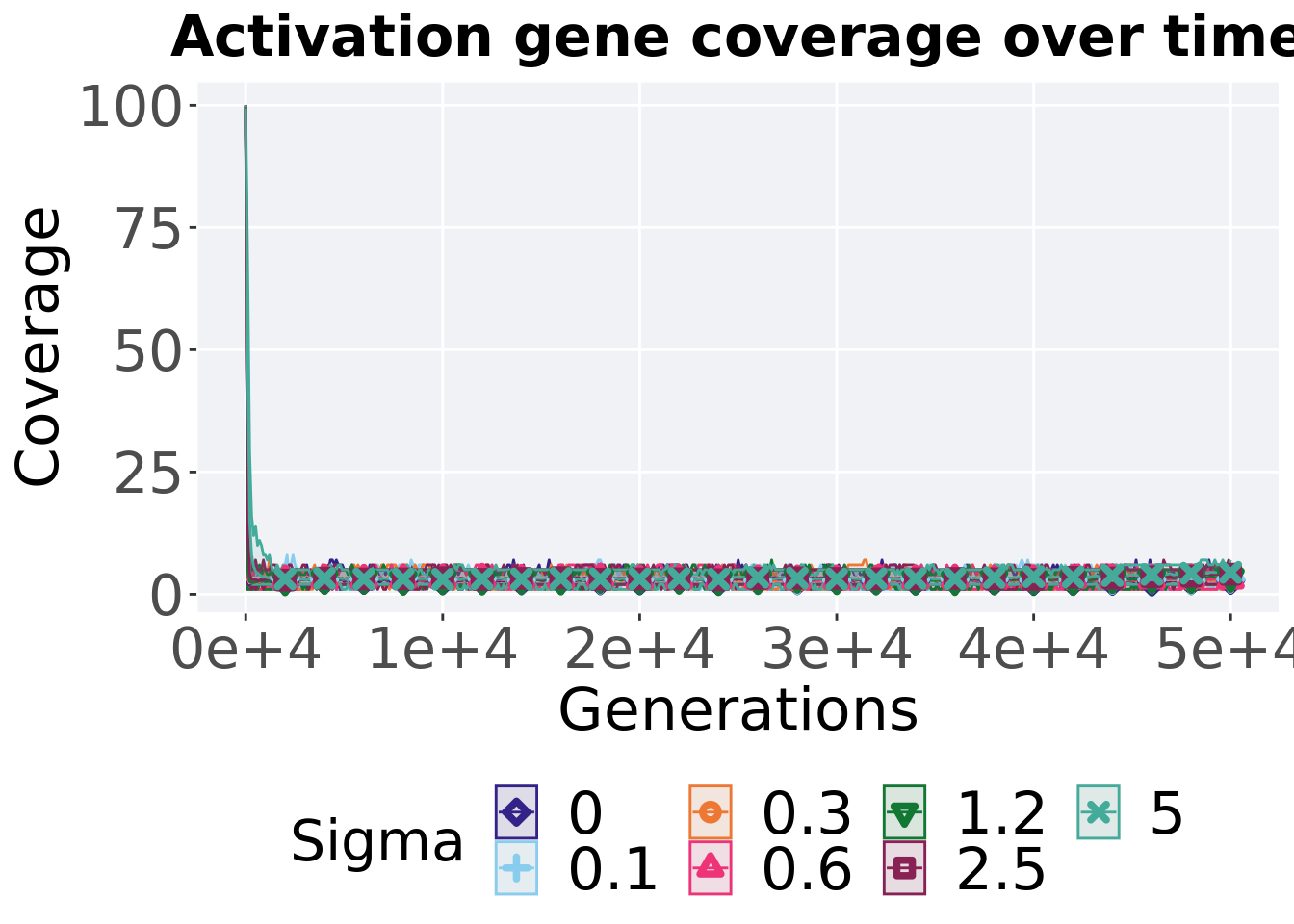

8.4.3.4 Activation gene coverage comparison

Best performances in the population at 40,000 and 50,000 generations.

# 80% and final generation comparison
end = filter(gfs_ot_mvc, diagnostic == 'multipath_exploration' & gen == 50000)
end$Generation <- factor(end$gen)

mid = filter(gfs_ot_mvc, diagnostic == 'multipath_exploration' & gen == 40000)
mid$Generation <- factor(mid$gen)

mvc_p = ggplot(mid, aes(x = Sigma, y=uni_str_pos, group = Sigma, shape = Generation)) +
  geom_point(col = mvc_col[1] , position = position_jitternudge(jitter.width = .03, nudge.x = -0.05), size = 2, alpha = 1.0) +
  geom_boxplot(position = position_nudge(x = -.15, y = 0), lwd = 0.7, col = mvc_col[1], fill = mvc_col[1], width = .1, outlier.shape = NA, alpha = 0.0) +

  geom_point(data = end, aes(x = Sigma, y=uni_str_pos), col = mvc_col[2], position = position_jitternudge(jitter.width = .03, nudge.x = 0.05), size = 2, alpha = 1.0) +
  geom_boxplot(data = end, aes(x = Sigma, y=uni_str_pos), position = position_nudge(x = .15, y = 0), lwd = 0.7, col = mvc_col[2], fill = mvc_col[2], width = .1, outlier.shape = NA, alpha = 0.0) +

  scale_y_continuous(
    name="Coverage",
  ) +
  scale_x_discrete(
    name="Sigma"
  )+
  scale_shape_manual(values=c(0,1))+
  scale_colour_manual(values = c(mvc_col[1],mvc_col[2])) +
  p_theme

plot_grid(
  mvc_p +
    ggtitle("Activation gene coverage over time") +
    theme(legend.position="none"),
  legend,
  nrow=2,
  rel_heights = c(1,.05),
  label_size = TSIZE
)

8.4.3.4.1 Stats

Summary statistics for the performance of the best performance at 40,000 and 50,000 generations.

slices = filter(gfs_ot_mvc, diagnostic == 'multipath_exploration' & (gen == 50000 | gen == 40000))
slices$Generation <- factor(slices$gen, levels = c(50000,40000))
slices %>%
  group_by(Sigma, Generation) %>%
  dplyr::summarise(
    count = n(),
    na_cnt = sum(is.na(uni_str_pos)),
    min = min(uni_str_pos, na.rm = TRUE),
    median = median(uni_str_pos, na.rm = TRUE),
    mean = mean(uni_str_pos, na.rm = TRUE),
    max = max(uni_str_pos, na.rm = TRUE),
    IQR = IQR(uni_str_pos, na.rm = TRUE)
  )

## `summarise()` has grouped output by 'Sigma'. You can override using the
## `.groups` argument.

## # A tibble: 14 x 9
## # Groups:   Sigma [7]
##    Sigma Generation count na_cnt   min median  mean   max   IQR
##    <fct> <fct>      <int>  <int> <int>  <dbl> <dbl> <int> <dbl>
##  1 0     50000         50      0     2      3  2.86     5  1.75
##  2 0     40000         50      0     1      3  2.62     4  1   
##  3 0.1   50000         50      0     1      3  3.1      5  1   
##  4 0.1   40000         50      0     2      3  2.86     6  1   
##  5 0.3   50000         50      0     2      3  3.14     5  1   
##  6 0.3   40000         50      0     1      3  2.72     4  1   
##  7 0.6   50000         50      0     1      3  2.92     5  1   
##  8 0.6   40000         50      0     1      3  2.88     5  1   
##  9 1.2   50000         50      0     2      4  3.5      5  1   
## 10 1.2   40000         50      0     2      3  3        5  1   
## 11 2.5   50000         50      0     2      4  4.1      6  2   
## 12 2.5   40000         50      0     2      3  3.04     5  0.75
## 13 5     50000         50      0     3      4  4.48     7  1   
## 14 5     40000         50      0     2      4  3.6      5  1

Sigma 0.0

wilcox.test(x = filter(slices, Sigma == 0.0 & Generation == 50000)$uni_str_pos,
            y = filter(slices, Sigma == 0.0 & Generation == 40000)$uni_str_pos,
            alternative = 't')

## 
##  Wilcoxon rank sum test with continuity correction
## 
## data:  filter(slices, Sigma == 0 & Generation == 50000)$uni_str_pos and filter(slices, Sigma == 0 & Generation == 40000)$uni_str_pos
## W = 1366, p-value = 0.3922
## alternative hypothesis: true location shift is not equal to 0

Sigma 0.1

wilcox.test(x = filter(slices, Sigma == 0.1 & Generation == 50000)$uni_str_pos,
            y = filter(slices, Sigma == 0.1 & Generation == 40000)$uni_str_pos,
            alternative = 't')

## 
##  Wilcoxon rank sum test with continuity correction
## 
## data:  filter(slices, Sigma == 0.1 & Generation == 50000)$uni_str_pos and filter(slices, Sigma == 0.1 & Generation == 40000)$uni_str_pos
## W = 1498.5, p-value = 0.07098
## alternative hypothesis: true location shift is not equal to 0

Sigma 0.3

wilcox.test(x = filter(slices, Sigma == 0.3 & Generation == 50000)$uni_str_pos,
            y = filter(slices, Sigma == 0.3 & Generation == 40000)$uni_str_pos,
            alternative = 't')

## 
##  Wilcoxon rank sum test with continuity correction
## 
## data:  filter(slices, Sigma == 0.3 & Generation == 50000)$uni_str_pos and filter(slices, Sigma == 0.3 & Generation == 40000)$uni_str_pos
## W = 1573, p-value = 0.01769
## alternative hypothesis: true location shift is not equal to 0

Sigma 0.6

wilcox.test(x = filter(slices, Sigma == 0.6 & Generation == 50000)$uni_str_pos,
            y = filter(slices, Sigma == 0.6 & Generation == 40000)$uni_str_pos,
            alternative = 't')

## 
##  Wilcoxon rank sum test with continuity correction
## 
## data:  filter(slices, Sigma == 0.6 & Generation == 50000)$uni_str_pos and filter(slices, Sigma == 0.6 & Generation == 40000)$uni_str_pos
## W = 1245.5, p-value = 0.9763
## alternative hypothesis: true location shift is not equal to 0

Sigma 1.2

wilcox.test(x = filter(slices, Sigma == 1.2 & Generation == 50000)$uni_str_pos,
            y = filter(slices, Sigma == 1.2 & Generation == 40000)$uni_str_pos,
            alternative = 't')

## 
##  Wilcoxon rank sum test with continuity correction
## 
## data:  filter(slices, Sigma == 1.2 & Generation == 50000)$uni_str_pos and filter(slices, Sigma == 1.2 & Generation == 40000)$uni_str_pos
## W = 1661.5, p-value = 0.002736
## alternative hypothesis: true location shift is not equal to 0

Sigma 2.5

wilcox.test(x = filter(slices, Sigma == 2.5 & Generation == 50000)$uni_str_pos,
            y = filter(slices, Sigma == 2.5 & Generation == 40000)$uni_str_pos,
            alternative = 't')

## 
##  Wilcoxon rank sum test with continuity correction
## 
## data:  filter(slices, Sigma == 2.5 & Generation == 50000)$uni_str_pos and filter(slices, Sigma == 2.5 & Generation == 40000)$uni_str_pos
## W = 1948, p-value = 4.828e-07
## alternative hypothesis: true location shift is not equal to 0

Sigma 5.0

wilcox.test(x = filter(slices, Sigma == 5.0 & Generation == 50000)$uni_str_pos,
            y = filter(slices, Sigma == 5.0 & Generation == 40000)$uni_str_pos,
            alternative = 't')

## 
##  Wilcoxon rank sum test with continuity correction
## 
## data:  filter(slices, Sigma == 5 & Generation == 50000)$uni_str_pos and filter(slices, Sigma == 5 & Generation == 40000)$uni_str_pos
## W = 1874.5, p-value = 4.82e-06
## alternative hypothesis: true location shift is not equal to 0