Chapter 11 Novelty Search
We present the results from our parameter sweep on novelty search.
50 replicates are conducted for each K-nearest neighbors parameter value explored.
11.1 Exploitation rate results
Here we present the results for best performances found by each novelty search K value replicate on the exploitation rate diagnostic. Best performance found refers to the largest average trait score found in a given population. Note that performance values fall between 0 and 100.
11.1.1 Performance over time
Performance over time.
lines = filter(nov_ot, diagnostic == 'exploitation_rate') %>%
        group_by(K, gen) %>%
          dplyr::summarise(
            min = min(pop_fit_max),
            mean = mean(pop_fit_max),
            max = max(pop_fit_max)
          )
## `summarise()` has grouped output by 'K'. You can override using the `.groups`
## argument.ggplot(lines, aes(x=gen, y=mean / DIMENSIONALITY, group = K, fill = K, color = K, shape = K)) +
geom_ribbon(aes(ymin = min / DIMENSIONALITY, ymax = max / DIMENSIONALITY), alpha = 0.1) +
geom_line(size = 0.5) +
geom_point(data = filter(lines, gen %% 2000 == 0 & gen != 0), size = 1.5, stroke = 2.0, alpha = 1.0) +
scale_y_continuous(
name="Average trait score"
) +
scale_x_continuous(
name="Generations",
limits=c(0, 50000),
breaks=c(0, 10000, 20000, 30000, 40000, 50000),
labels=c("0e+4", "1e+4", "2e+4", "3e+4", "4e+4", "5e+4")
) +
scale_shape_manual(values=SHAPE)+
scale_colour_manual(values = cb_palette) +
scale_fill_manual(values = cb_palette) +
ggtitle("Best performance over time") +
p_theme
11.1.2 Best performance throughout
The best performance found throughout 50,000 generations.
filter(nov_best, col == 'pop_fit_max' &  diagnostic == 'exploitation_rate') %>%
ggplot(., aes(x = K, y = val / DIMENSIONALITY, color = K, fill = K, shape = K)) +
  geom_flat_violin(position = position_nudge(x = .2, y = 0), scale = 'width', alpha = 0.2) +
  geom_point(position = position_jitter(width = .1), size = 1.5, alpha = 1.0) +
  geom_boxplot(color = 'black', width = .2, outlier.shape = NA, alpha = 0.0) +
  scale_y_continuous(
    name="Average trait score"
  ) +
  scale_x_discrete(
    name="K"
  )+
  scale_shape_manual(values=SHAPE)+
  scale_colour_manual(values = cb_palette) +
  scale_fill_manual(values = cb_palette) +
    ggtitle("Best performance throughout") +
  p_theme
11.1.2.1 Stats
Summary statistics for the best performance found throughout 50,000 generations.
performance = filter(nov_best, col == 'pop_fit_max' & diagnostic == 'exploitation_rate');
group_by(performance, K) %>%
  dplyr::summarise(
    count = n(),
    na_cnt = sum(is.na(val)),
    min = min(val / DIMENSIONALITY, na.rm = TRUE),
    median = median(val / DIMENSIONALITY, na.rm = TRUE),
    mean = mean(val / DIMENSIONALITY, na.rm = TRUE),
    max = max(val / DIMENSIONALITY, na.rm = TRUE),
    IQR = IQR(val / DIMENSIONALITY, na.rm = TRUE)
  )
## # A tibble: 6 x 8
## K count na_cnt min median mean max IQR
## <fct> <int> <int> <dbl> <dbl> <dbl> <dbl> <dbl>
## 1 1 50 0 16.8 20.3 20.1 23.2 2.72
## 2 2 50 0 17.3 20.1 20.2 22.6 1.98
## 3 4 50 0 17.2 20.8 20.6 23.1 1.34
## 4 8 50 0 17.3 20.1 20.2 23.4 1.42
## 5 15 50 0 15.9 19.2 19.3 22.3 1.34
## 6 30 50 0 16.8 19.2 19.2 21.8 1.44Kruskal–Wallis test provides evidence of significant differences among K values on the best performance found throughout 50,000 generations
##
##  Kruskal-Wallis rank sum test
##
## data:  val by K
## Kruskal-Wallis chi-squared = 41.239, df = 5, p-value = 8.394e-08
Results for post-hoc Wilcoxon rank-sum test with a Bonferroni correction on the best performance found throughout 50,000 generations.
pairwise.wilcox.test(x = performance$val, g = performance$K , p.adjust.method = "bonferroni",
                     paired = FALSE, conf.int = FALSE, alternative = 't')
##
## Pairwise comparisons using Wilcoxon rank sum test with continuity correction
##
## data: performance$val and performance$K
##
## 1 2 4 8 15
## 2 1.0000 - - - -
## 4 1.0000 1.0000 - - -
## 8 1.0000 1.0000 0.5941 - -
## 15 0.1905 0.0068 3.9e-05 0.0072 -
## 30 0.0777 0.0023 6.2e-06 0.0025 1.0000
##
## P value adjustment method: bonferroni11.1.3 Multi-valley crossing
11.1.3.1 Performance over time
# data for lines and shading on plots
lines = filter(nov_ot_mvc, diagnostic == 'exploitation_rate') %>%
  group_by(K, gen) %>%
  dplyr::summarise(
    min = min(pop_fit_max) / DIMENSIONALITY,
    mean = mean(pop_fit_max) / DIMENSIONALITY,
    max = max(pop_fit_max) / DIMENSIONALITY
  )
## `summarise()` has grouped output by 'K'. You can override using the `.groups`
## argument.ggplot(lines, aes(x=gen, y=mean, group = K, fill =K, color = K, shape = K)) +
geom_ribbon(aes(ymin = min, ymax = max), alpha = 0.1) +
geom_line(size = 0.5) +
geom_point(data = filter(lines, gen %% 2000 == 0 & gen != 0), size = 1.5, stroke = 2.0, alpha = 1.0) +
scale_y_continuous(
name="Average trait score"
) +
scale_x_continuous(
name="Generations",
limits=c(0, 50000),
breaks=c(0, 10000, 20000, 30000, 40000, 50000),
labels=c("0e+4", "1e+4", "2e+4", "3e+4", "4e+4", "5e+4")
) +
scale_shape_manual(values=SHAPE)+
scale_colour_manual(values = cb_palette) +
scale_fill_manual(values = cb_palette) +
ggtitle('Performance over time')+
p_theme
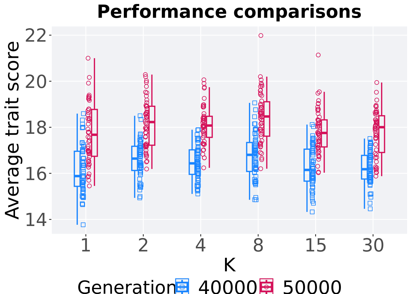
11.1.3.2 Performance comparison
Best performances in the population at 40,000 and 50,000 generations.
# 80% and final generation comparison
end = filter(nov_ot_mvc, diagnostic == 'exploitation_rate' & gen == 50000)
end$Generation <- factor(end$gen)

mid = filter(nov_ot_mvc, diagnostic == 'exploitation_rate' & gen == 40000)
mid$Generation <- factor(mid$gen)

mvc_p = ggplot(mid, aes(x = K, y=pop_fit_max / DIMENSIONALITY, group = K, shape = Generation)) +
  geom_point(col = mvc_col[1] , position = position_jitternudge(jitter.width = .03, nudge.x = -0.05), size = 2, alpha = 1.0) +
  geom_boxplot(position = position_nudge(x = -.15, y = 0), lwd = 0.7, col = mvc_col[1], fill = mvc_col[1], width = .1, outlier.shape = NA, alpha = 0.0) +

  geom_point(data = end, aes(x = K, y=pop_fit_max / DIMENSIONALITY), col = mvc_col[2], position = position_jitternudge(jitter.width = .03, nudge.x = 0.05), size = 2, alpha = 1.0) +
  geom_boxplot(data = end, aes(x = K, y=pop_fit_max / DIMENSIONALITY), position = position_nudge(x = .15, y = 0), lwd = 0.7, col = mvc_col[2], fill = mvc_col[2], width = .1, outlier.shape = NA, alpha = 0.0) +

  scale_y_continuous(
    name="Average trait score"
  ) +
  scale_x_discrete(
    name="K"
  )+
  scale_shape_manual(values=c(0,1))+
  scale_colour_manual(values = c(mvc_col[1],mvc_col[2])) +
  p_theme

plot_grid(
  mvc_p +
    ggtitle("Performance comparisons") +
    theme(legend.position="none"),
  legend,
  nrow=2,
  rel_heights = c(1,.05),
  label_size = TSIZE
)
11.1.3.3 Stats
Summary statistics for the performance of the best performance at 40,000 and 50,000 generations.
slices = filter(nov_ot_mvc, diagnostic == 'exploitation_rate' & (gen == 50000 | gen == 40000))
slices$Generation <- factor(slices$gen, levels = c(50000,40000))
slices %>%
  group_by(K, Generation) %>%
  dplyr::summarise(
    count = n(),
    na_cnt = sum(is.na(pop_fit_max  / DIMENSIONALITY)),
    min = min(pop_fit_max  / DIMENSIONALITY, na.rm = TRUE),
    median = median(pop_fit_max  / DIMENSIONALITY, na.rm = TRUE),
    mean = mean(pop_fit_max  / DIMENSIONALITY, na.rm = TRUE),
    max = max(pop_fit_max  / DIMENSIONALITY, na.rm = TRUE),
    IQR = IQR(pop_fit_max  / DIMENSIONALITY, na.rm = TRUE)
  )
## `summarise()` has grouped output by 'K'. You can override using the `.groups`
## argument.## # A tibble: 12 x 9
## # Groups: K [6]
## K Generation count na_cnt min median mean max IQR
## <fct> <fct> <int> <int> <dbl> <dbl> <dbl> <dbl> <dbl>
## 1 1 50000 50 0 15.5 17.7 17.7 21.0 2.03
## 2 1 40000 50 0 13.8 15.9 16.1 18.6 1.52
## 3 2 50000 50 0 16.2 18.2 18.2 20.3 1.69
## 4 2 40000 50 0 14.9 16.6 16.6 18.5 1.05
## 5 4 50000 50 0 16.2 18.1 18.1 20.1 0.914
## 6 4 40000 50 0 15.1 16.4 16.5 17.9 1.06
## 7 8 50000 50 0 16.2 18.5 18.4 22.0 1.49
## 8 8 40000 50 0 14.9 16.8 16.7 19.1 1.26
## 9 15 50000 50 0 16.0 17.8 17.8 21.1 1.17
## 10 15 40000 50 0 14.3 16.1 16.3 18.1 1.39
## 11 30 50000 50 0 15.9 18.0 17.8 19.9 1.59
## 12 30 40000 50 0 14.5 16.2 16.2 17.5 1.03K 1
wilcox.test(x = filter(slices, K == 1 & Generation == 50000)$pop_fit_max,
            y = filter(slices, K == 1 & Generation == 40000)$pop_fit_max,
            alternative = 't')
##
## Wilcoxon rank sum test with continuity correction
##
## data: filter(slices, K == 1 & Generation == 50000)$pop_fit_max and filter(slices, K == 1 & Generation == 40000)$pop_fit_max
## W = 2073, p-value = 1.427e-08
## alternative hypothesis: true location shift is not equal to 0K 2
wilcox.test(x = filter(slices, K == 2 & Generation == 50000)$pop_fit_max,
            y = filter(slices, K == 2 & Generation == 40000)$pop_fit_max,
            alternative = 't')
##
## Wilcoxon rank sum test with continuity correction
##
## data: filter(slices, K == 2 & Generation == 50000)$pop_fit_max and filter(slices, K == 2 & Generation == 40000)$pop_fit_max
## W = 2191, p-value = 8.954e-11
## alternative hypothesis: true location shift is not equal to 0K 4
wilcox.test(x = filter(slices, K == 4 & Generation == 50000)$pop_fit_max,
            y = filter(slices, K == 4 & Generation == 40000)$pop_fit_max,
            alternative = 't')
##
## Wilcoxon rank sum test with continuity correction
##
## data: filter(slices, K == 4 & Generation == 50000)$pop_fit_max and filter(slices, K == 4 & Generation == 40000)$pop_fit_max
## W = 2315, p-value = 2.16e-13
## alternative hypothesis: true location shift is not equal to 0K 8
wilcox.test(x = filter(slices, K == 8 & Generation == 50000)$pop_fit_max,
            y = filter(slices, K == 8 & Generation == 40000)$pop_fit_max,
            alternative = 't')
##
## Wilcoxon rank sum test with continuity correction
##
## data: filter(slices, K == 8 & Generation == 50000)$pop_fit_max and filter(slices, K == 8 & Generation == 40000)$pop_fit_max
## W = 2178, p-value = 1.616e-10
## alternative hypothesis: true location shift is not equal to 0K 15
wilcox.test(x = filter(slices, K == 15 & Generation == 50000)$pop_fit_max,
            y = filter(slices, K == 15 & Generation == 40000)$pop_fit_max,
            alternative = 't')
##
## Wilcoxon rank sum test with continuity correction
##
## data: filter(slices, K == 15 & Generation == 50000)$pop_fit_max and filter(slices, K == 15 & Generation == 40000)$pop_fit_max
## W = 2196, p-value = 7.119e-11
## alternative hypothesis: true location shift is not equal to 0K 30
wilcox.test(x = filter(slices, K == 30 & Generation == 50000)$pop_fit_max,
            y = filter(slices, K == 30 & Generation == 40000)$pop_fit_max,
            alternative = 't')
##
## Wilcoxon rank sum test with continuity correction
##
## data: filter(slices, K == 30 & Generation == 50000)$pop_fit_max and filter(slices, K == 30 & Generation == 40000)$pop_fit_max
## W = 2200, p-value = 5.922e-11
## alternative hypothesis: true location shift is not equal to 011.2 Ordered exploitation results
Here we present the results for best performances found by each novelty search K value replicate on the ordered exploitation diagnostic. Best performance found refers to the largest average trait score found in a given population. Note that performance values fall between 0 and 100.
11.2.1 Performance over time
Performance over time.
lines = filter(nov_ot, diagnostic == 'ordered_exploitation') %>%
        group_by(K, gen) %>%
          dplyr::summarise(
            min = min(pop_fit_max),
            mean = mean(pop_fit_max),
            max = max(pop_fit_max)
          )
## `summarise()` has grouped output by 'K'. You can override using the `.groups`
## argument.ggplot(lines, aes(x=gen, y=mean / DIMENSIONALITY, group = K, fill = K, color = K, shape = K)) +
geom_ribbon(aes(ymin = min / DIMENSIONALITY, ymax = max / DIMENSIONALITY), alpha = 0.1) +
geom_line(size = 0.5) +
geom_point(data = filter(lines, gen %% 2000 == 0 & gen != 0), size = 1.5, stroke = 2.0, alpha = 1.0) +
scale_y_continuous(
name="Average trait score"
) +
scale_x_continuous(
name="Generations",
limits=c(0, 50000),
breaks=c(0, 10000, 20000, 30000, 40000, 50000),
labels=c("0e+4", "1e+4", "2e+4", "3e+4", "4e+4", "5e+4")
) +
scale_shape_manual(values=SHAPE)+
scale_colour_manual(values = cb_palette) +
scale_fill_manual(values = cb_palette) +
ggtitle("Best performance over time") +
p_theme
11.2.2 Best performance throughout
The best performance found throughout 50,000 generations.
filter(nov_best, col == 'pop_fit_max' & diagnostic == 'ordered_exploitation') %>%
ggplot(., aes(x = K, y = val / DIMENSIONALITY, color = K, fill = K, shape = K)) +
  geom_flat_violin(position = position_nudge(x = .2, y = 0), scale = 'width', alpha = 0.2) +
  geom_point(position = position_jitter(width = .1), size = 1.5, alpha = 1.0) +
  geom_boxplot(color = 'black', width = .2, outlier.shape = NA, alpha = 0.0) +
  scale_y_continuous(
    name="Average trait score"
  ) +
  scale_x_discrete(
    name="K"
  )+
  scale_shape_manual(values = SHAPE)+
  scale_colour_manual(values = cb_palette) +
  scale_fill_manual(values = cb_palette) +
  ggtitle("Best performance throughout") +
  p_theme
11.2.2.1 Stats
Summary statistics about the best performance found.
performance = filter(nov_best, col == 'pop_fit_max' & diagnostic == 'ordered_exploitation')
group_by(performance, K) %>%
  dplyr::summarise(
    count = n(),
    na_cnt = sum(is.na(val)),
    min = min(val / DIMENSIONALITY, na.rm = TRUE),
    median = median(val / DIMENSIONALITY, na.rm = TRUE),
    mean = mean(val / DIMENSIONALITY, na.rm = TRUE),
    max = max(val / DIMENSIONALITY, na.rm = TRUE),
    IQR = IQR(val / DIMENSIONALITY, na.rm = TRUE)
  )
## # A tibble: 6 x 8
## K count na_cnt min median mean max IQR
## <fct> <int> <int> <dbl> <dbl> <dbl> <dbl> <dbl>
## 1 1 50 0 2.27 3.81 3.89 5.35 1.06
## 2 2 50 0 2.83 4.88 4.92 6.54 0.928
## 3 4 50 0 3.79 5.43 5.46 6.94 1.09
## 4 8 50 0 3.61 4.58 4.58 5.80 0.826
## 5 15 50 0 2.55 3.70 3.80 5.82 0.718
## 6 30 50 0 3.05 4.99 5.00 7.28 0.835Kruskal–Wallis test provides evidence of statistical differences for the best performance found in the pouplation throughout 50,000 generations.
##
##  Kruskal-Wallis rank sum test
##
## data:  val by K
## Kruskal-Wallis chi-squared = 127.68, df = 5, p-value < 2.2e-16
Results for post-hoc Wilcoxon rank-sum test with a Bonferroni correction on the best performance found in the pouplation throughout 50,000 generations.
pairwise.wilcox.test(x = performance$val, g = performance$K , p.adjust.method = "bonferroni",
                     paired = FALSE, conf.int = FALSE, alternative = 't')
##
## Pairwise comparisons using Wilcoxon rank sum test with continuity correction
##
## data: performance$val and performance$K
##
## 1 2 4 8 15
## 2 5.1e-08 - - - -
## 4 6.3e-12 0.02655 - - -
## 8 0.00017 0.11567 1.1e-06 - -
## 15 1.00000 2.9e-10 1.5e-13 5.5e-08 -
## 30 8.4e-08 1.00000 0.10010 0.03273 4.9e-10
##
## P value adjustment method: bonferroni11.2.3 Multi-valley crossing
11.2.3.1 Performance over time
# data for lines and shading on plots
lines = filter(nov_ot_mvc, diagnostic == 'ordered_exploitation') %>%
  group_by(K, gen) %>%
  dplyr::summarise(
    min = min(pop_fit_max) / DIMENSIONALITY,
    mean = mean(pop_fit_max) / DIMENSIONALITY,
    max = max(pop_fit_max) / DIMENSIONALITY
  )
## `summarise()` has grouped output by 'K'. You can override using the `.groups`
## argument.ggplot(lines, aes(x=gen, y=mean, group = K, fill =K, color = K, shape = K)) +
geom_ribbon(aes(ymin = min, ymax = max), alpha = 0.1) +
geom_line(size = 0.5) +
geom_point(data = filter(lines, gen %% 2000 == 0 & gen != 0), size = 1.5, stroke = 2.0, alpha = 1.0) +
scale_y_continuous(
name="Average trait score"
) +
scale_x_continuous(
name="Generations",
limits=c(0, 50000),
breaks=c(0, 10000, 20000, 30000, 40000, 50000),
labels=c("0e+4", "1e+4", "2e+4", "3e+4", "4e+4", "5e+4")
) +
scale_shape_manual(values=SHAPE)+
scale_colour_manual(values = cb_palette) +
scale_fill_manual(values = cb_palette) +
ggtitle('Performance over time')+
p_theme
11.2.3.2 Performance comparison
Best performances in the population at 40,000 and 50,000 generations.
# 80% and final generation comparison
end = filter(nov_ot_mvc, diagnostic == 'ordered_exploitation' & gen == 50000)
end$Generation <- factor(end$gen)

mid = filter(nov_ot_mvc, diagnostic == 'ordered_exploitation' & gen == 40000)
mid$Generation <- factor(mid$gen)

mvc_p = ggplot(mid, aes(x = K, y=pop_fit_max / DIMENSIONALITY, group = K, shape = Generation)) +
  geom_point(col = mvc_col[1] , position = position_jitternudge(jitter.width = .03, nudge.x = -0.05), size = 2, alpha = 1.0) +
  geom_boxplot(position = position_nudge(x = -.15, y = 0), lwd = 0.7, col = mvc_col[1], fill = mvc_col[1], width = .1, outlier.shape = NA, alpha = 0.0) +

  geom_point(data = end, aes(x = K, y=pop_fit_max / DIMENSIONALITY), col = mvc_col[2], position = position_jitternudge(jitter.width = .03, nudge.x = 0.05), size = 2, alpha = 1.0) +
  geom_boxplot(data = end, aes(x = K, y=pop_fit_max / DIMENSIONALITY), position = position_nudge(x = .15, y = 0), lwd = 0.7, col = mvc_col[2], fill = mvc_col[2], width = .1, outlier.shape = NA, alpha = 0.0) +

  scale_y_continuous(
    name="Average trait score"
  ) +
  scale_x_discrete(
    name="K"
  )+
  scale_shape_manual(values=c(0,1))+
  scale_colour_manual(values = c(mvc_col[1],mvc_col[2])) +
  p_theme

plot_grid(
  mvc_p +
    ggtitle("Performance comparisons") +
    theme(legend.position="none"),
  legend,
  nrow=2,
  rel_heights = c(1,.05),
  label_size = TSIZE
)
11.2.3.3 Stats
Summary statistics for the performance of the best performance at 40,000 and 50,000 generations.
slices = filter(nov_ot_mvc, diagnostic == 'ordered_exploitation' & (gen == 50000 | gen == 40000))
slices$Generation <- factor(slices$gen, levels = c(50000,40000))
slices %>%
  group_by(K, Generation) %>%
  dplyr::summarise(
    count = n(),
    na_cnt = sum(is.na(pop_fit_max  / DIMENSIONALITY)),
    min = min(pop_fit_max  / DIMENSIONALITY, na.rm = TRUE),
    median = median(pop_fit_max  / DIMENSIONALITY, na.rm = TRUE),
    mean = mean(pop_fit_max  / DIMENSIONALITY, na.rm = TRUE),
    max = max(pop_fit_max  / DIMENSIONALITY, na.rm = TRUE),
    IQR = IQR(pop_fit_max  / DIMENSIONALITY, na.rm = TRUE)
  )
## `summarise()` has grouped output by 'K'. You can override using the `.groups`
## argument.## # A tibble: 12 x 9
## # Groups: K [6]
## K Generation count na_cnt min median mean max IQR
## <fct> <fct> <int> <int> <dbl> <dbl> <dbl> <dbl> <dbl>
## 1 1 50000 50 0 1.92 3.21 3.24 5.16 0.666
## 2 1 40000 50 0 1.84 2.72 2.83 4.11 0.569
## 3 2 50000 50 0 2.56 4.21 4.10 5.86 0.669
## 4 2 40000 50 0 2.40 3.57 3.61 4.99 0.710
## 5 4 50000 50 0 1.89 3.91 3.97 5.15 0.720
## 6 4 40000 50 0 2.00 3.56 3.51 4.51 0.527
## 7 8 50000 50 0 2.15 3.15 3.12 4.00 0.448
## 8 8 40000 50 0 1.99 2.97 2.92 3.72 0.448
## 9 15 50000 50 0 2.35 3.43 3.38 4.38 0.670
## 10 15 40000 50 0 2.27 3.06 3.03 3.99 0.560
## 11 30 50000 50 0 3.77 4.45 4.54 5.88 0.789
## 12 30 40000 50 0 3.20 4.06 4.10 5.41 0.582K 1
wilcox.test(x = filter(slices, K == 1 & Generation == 50000)$pop_fit_max,
            y = filter(slices, K == 1 & Generation == 40000)$pop_fit_max,
            alternative = 't')
##
## Wilcoxon rank sum test with continuity correction
##
## data: filter(slices, K == 1 & Generation == 50000)$pop_fit_max and filter(slices, K == 1 & Generation == 40000)$pop_fit_max
## W = 1779, p-value = 0.0002691
## alternative hypothesis: true location shift is not equal to 0K 2
wilcox.test(x = filter(slices, K == 2 & Generation == 50000)$pop_fit_max,
            y = filter(slices, K == 2 & Generation == 40000)$pop_fit_max,
            alternative = 't')
##
## Wilcoxon rank sum test with continuity correction
##
## data: filter(slices, K == 2 & Generation == 50000)$pop_fit_max and filter(slices, K == 2 & Generation == 40000)$pop_fit_max
## W = 1809, p-value = 0.000118
## alternative hypothesis: true location shift is not equal to 0K 4
wilcox.test(x = filter(slices, K == 4 & Generation == 50000)$pop_fit_max,
            y = filter(slices, K == 4 & Generation == 40000)$pop_fit_max,
            alternative = 't')
##
## Wilcoxon rank sum test with continuity correction
##
## data: filter(slices, K == 4 & Generation == 50000)$pop_fit_max and filter(slices, K == 4 & Generation == 40000)$pop_fit_max
## W = 1889, p-value = 1.074e-05
## alternative hypothesis: true location shift is not equal to 0K 8
wilcox.test(x = filter(slices, K == 8 & Generation == 50000)$pop_fit_max,
            y = filter(slices, K == 8 & Generation == 40000)$pop_fit_max,
            alternative = 't')
##
## Wilcoxon rank sum test with continuity correction
##
## data: filter(slices, K == 8 & Generation == 50000)$pop_fit_max and filter(slices, K == 8 & Generation == 40000)$pop_fit_max
## W = 1608, p-value = 0.01372
## alternative hypothesis: true location shift is not equal to 0K 15
wilcox.test(x = filter(slices, K == 15 & Generation == 50000)$pop_fit_max,
            y = filter(slices, K == 15 & Generation == 40000)$pop_fit_max,
            alternative = 't')
##
## Wilcoxon rank sum test with continuity correction
##
## data: filter(slices, K == 15 & Generation == 50000)$pop_fit_max and filter(slices, K == 15 & Generation == 40000)$pop_fit_max
## W = 1789, p-value = 0.0002054
## alternative hypothesis: true location shift is not equal to 0K 30
wilcox.test(x = filter(slices, K == 30 & Generation == 50000)$pop_fit_max,
            y = filter(slices, K == 30 & Generation == 40000)$pop_fit_max,
            alternative = 't')
##
## Wilcoxon rank sum test with continuity correction
##
## data: filter(slices, K == 30 & Generation == 50000)$pop_fit_max and filter(slices, K == 30 & Generation == 40000)$pop_fit_max
## W = 1799, p-value = 0.000156
## alternative hypothesis: true location shift is not equal to 011.3 Contraditory objectives diagnostic
Here we present the results for satisfactory trait coverage and activation gene coverage found by each novelty search K value replicate on the contradictory objectives diagnostic. Satisfactory trait coverage refers to the count of unique satisfied traits in the population, while activation gene coverage refers to the count of unique activation genes in the population. Note that both coverage values fall between 0 and 100.
11.3.1 Satisfactory trait coverage
Here we analyze the satisfactory trait coverage for each parameter replicate on the contradictory objectives diagnostic.
11.3.1.1 Coverage over time
Satisfactory trait coverage over time.
lines = filter(nov_ot, diagnostic == 'contradictory_objectives') %>%
        group_by(K, gen) %>%
          dplyr::summarise(
            min = min(pop_uni_obj),
            mean = mean(pop_uni_obj),
            max = max(pop_uni_obj)
          )
## `summarise()` has grouped output by 'K'. You can override using the `.groups`
## argument.ggplot(lines, aes(x=gen, y=mean, group = K, fill =K, color = K, shape = K)) +
geom_ribbon(aes(ymin = min, ymax = max), alpha = 0.1) +
geom_line(size = 0.5) +
geom_point(data = filter(lines, gen %% 2000 == 0 & gen != 0), size = 1.5, stroke = 2.0, alpha = 1.0) +
scale_y_continuous(
name="Coverage"
) +
scale_x_continuous(
name="Generations",
limits=c(0, 50000),
breaks=c(0, 10000, 20000, 30000, 40000, 50000),
labels=c("0e+4", "1e+4", "2e+4", "3e+4", "4e+4", "5e+4")
) +
scale_shape_manual(values=SHAPE)+
scale_colour_manual(values = cb_palette) +
scale_fill_manual(values = cb_palette) +
ggtitle("Satisfactory trait coverage over time") +
p_theme
11.3.1.2 Best coverage throughout
Best satisfactory trait coverage throughout 50,000 generations.
filter(nov_best, col == 'pop_uni_obj' & diagnostic == 'contradictory_objectives') %>%
ggplot(., aes(x = K, y = val, color = K, fill = K, shape = K)) +
  geom_flat_violin(position = position_nudge(x = .2, y = 0), scale = 'width', alpha = 0.2) +
  geom_point(position = position_jitter(width = .1), size = 1.5, alpha = 1.0) +
  geom_boxplot(color = 'black', width = .2, outlier.shape = NA, alpha = 0.0) +
  scale_y_continuous(
    name="Coverage",
    limits=c(-1, 5)
  ) +
  scale_x_discrete(
    name="K"
  )+
  scale_shape_manual(values=SHAPE)+
  scale_colour_manual(values = cb_palette) +
  scale_fill_manual(values = cb_palette) +
  ggtitle("Best satisfactory trait coverage") +
  p_theme
11.3.1.2.1 Stats
Summary statistics for the best satisfactory trait coverage throughout 50,000 generations.
coverage = filter(nov_best, col == 'pop_uni_obj' & diagnostic == 'contradictory_objectives')
group_by(coverage, K) %>%
  dplyr::summarise(
    count = n(),
    na_cnt = sum(is.na(val)),
    min = min(val, na.rm = TRUE),
    median = median(val, na.rm = TRUE),
    mean = mean(val, na.rm = TRUE),
    max = max(val, na.rm = TRUE),
    IQR = IQR(val, na.rm = TRUE)
  )
## # A tibble: 6 x 8
## K count na_cnt min median mean max IQR
## <fct> <int> <int> <dbl> <dbl> <dbl> <dbl> <dbl>
## 1 1 50 0 0 0 0.02 1 0
## 2 2 50 0 0 0 0 0 0
## 3 4 50 0 0 0 0 0 0
## 4 8 50 0 0 0 0 0 0
## 5 15 50 0 0 0 0 0 0
## 6 30 50 0 0 0 0 0 011.3.1.3 End of 50,000 generations
Satisfactory trait coverage in the population at the end of 50,000 generations.
filter(nov_ot, diagnostic == 'contradictory_objectives' & gen == 50000) %>%
ggplot(., aes(x = K, y = pop_uni_obj, color = K, fill = K, shape = K)) +
  geom_flat_violin(position = position_nudge(x = .2, y = 0), scale = 'width', alpha = 0.2) +
  geom_point(position = position_jitter(width = .1), size = 1.5, alpha = 1.0) +
  geom_boxplot(color = 'black', width = .2, outlier.shape = NA, alpha = 0.0) +
  scale_y_continuous(
    name="Coverage",
    limits=c(-1, 5)
  ) +
  scale_x_discrete(
    name="K"
  )+
  scale_shape_manual(values=SHAPE)+
  scale_colour_manual(values = cb_palette) +
  scale_fill_manual(values = cb_palette) +
  ggtitle("Final satisfactory trait coverage") +
  p_theme
11.3.1.3.1 Stats
Summary statistics for satisfactory trait coverage in the population at the end of 50,000 generations.
coverage = filter(nov_ot, diagnostic == 'contradictory_objectives' & gen == 50000)
group_by(coverage, K) %>%
  dplyr::summarise(
    count = n(),
    na_cnt = sum(is.na(pop_uni_obj)),
    min = min(pop_uni_obj, na.rm = TRUE),
    median = median(pop_uni_obj, na.rm = TRUE),
    mean = mean(pop_uni_obj, na.rm = TRUE),
    max = max(pop_uni_obj, na.rm = TRUE),
    IQR = IQR(pop_uni_obj, na.rm = TRUE)
  )
## # A tibble: 6 x 8
## K count na_cnt min median mean max IQR
## <fct> <int> <int> <int> <dbl> <dbl> <int> <dbl>
## 1 1 50 0 0 0 0.02 1 0
## 2 2 50 0 0 0 0 0 0
## 3 4 50 0 0 0 0 0 0
## 4 8 50 0 0 0 0 0 0
## 5 15 50 0 0 0 0 0 0
## 6 30 50 0 0 0 0 0 011.3.2 Activation gene coverage
Here we analyze the activation gene coverage for each parameter replicate on the contradictory objectives diagnostic.
11.3.2.1 Coverage over time
Activation gene coverage over time.
lines = filter(nov_ot, diagnostic == 'contradictory_objectives') %>%
        group_by(K, gen) %>%
          dplyr::summarise(
            min = min(uni_str_pos),
            mean = mean(uni_str_pos),
            max = max(uni_str_pos)
          )
## `summarise()` has grouped output by 'K'. You can override using the `.groups`
## argument.ggplot(lines, aes(x=gen, y=mean, group = K, fill =K, color = K, shape = K)) +
geom_ribbon(aes(ymin = min, ymax = max), alpha = 0.1) +
geom_line(size = 0.5) +
geom_point(data = filter(lines, gen %% 2000 == 0 & gen != 0), size = 1.5, stroke = 2.0, alpha = 1.0) +
scale_y_continuous(
name="Coverage",
limits=c(-1, 101),
breaks=seq(0,100, 20),
labels=c("0", "20", "40", "60", "80", "100")
) +
scale_x_continuous(
name="Generations",
limits=c(0, 50000),
breaks=c(0, 10000, 20000, 30000, 40000, 50000),
labels=c("0e+4", "1e+4", "2e+4", "3e+4", "4e+4", "5e+4")
) +
scale_shape_manual(values=SHAPE)+
scale_colour_manual(values = cb_palette) +
scale_fill_manual(values = cb_palette) +
ggtitle("Activation gene coverage over time") +
p_theme
11.3.2.2 End of 50,000 generations
Activation gene coverage in the population at the end of 50,000 generations.
filter(nov_ot, diagnostic == 'contradictory_objectives' & gen == 50000) %>%
ggplot(., aes(x = K, y = uni_str_pos, color = K, fill = K, shape = K)) +
  geom_flat_violin(position = position_nudge(x = .2, y = 0), scale = 'width', alpha = 0.2) +
  geom_point(position = position_jitter(width = .1), size = 1.5, alpha = 1.0) +
  geom_boxplot(color = 'black', width = .2, outlier.shape = NA, alpha = 0.0) +
  scale_y_continuous(
    name="Coverage"
  ) +
  scale_x_discrete(
    name="K"
  )+
  scale_shape_manual(values=SHAPE)+
  scale_colour_manual(values = cb_palette) +
  scale_fill_manual(values = cb_palette) +
  ggtitle("Final activation gene coverage") +
  p_theme
11.3.2.2.1 Stats
Summary statistics for the activation gene coverage in the population at the end of 50,000 generations.
coverage = filter(nov_ot, diagnostic == 'contradictory_objectives' & gen == 50000)
group_by(coverage, K) %>%
  dplyr::summarise(
    count = n(),
    na_cnt = sum(is.na(uni_str_pos)),
    min = min(uni_str_pos, na.rm = TRUE),
    median = median(uni_str_pos, na.rm = TRUE),
    mean = mean(uni_str_pos, na.rm = TRUE),
    max = max(uni_str_pos, na.rm = TRUE),
    IQR = IQR(uni_str_pos, na.rm = TRUE)
  )
## # A tibble: 6 x 8
## K count na_cnt min median mean max IQR
## <fct> <int> <int> <int> <dbl> <dbl> <int> <dbl>
## 1 1 50 0 71 85 84.6 92 5
## 2 2 50 0 87 97 96.2 100 3
## 3 4 50 0 99 100 99.8 100 0
## 4 8 50 0 98 100 99.7 100 0.75
## 5 15 50 0 98 100 99.6 100 1
## 6 30 50 0 83 91 90.9 96 3Kruskal–Wallis test provides evidence of statistical differences among activation gene coverage in the population at the end of 50,000 generations.
##
##  Kruskal-Wallis rank sum test
##
## data:  uni_str_pos by K
## Kruskal-Wallis chi-squared = 260.74, df = 5, p-value < 2.2e-16
Results for post-hoc Wilcoxon rank-sum test with a Bonferroni correction on the activation gene coverage in the population at the end of 50,000 generations.
pairwise.wilcox.test(x = coverage$uni_str_pos, g = coverage$K , p.adjust.method = "bonferroni",
                     paired = FALSE, conf.int = FALSE, alternative = 't')
##
## Pairwise comparisons using Wilcoxon rank sum test with continuity correction
##
## data: coverage$uni_str_pos and coverage$K
##
## 1 2 4 8 15
## 2 4.4e-16 - - - -
## 4 < 2e-16 < 2e-16 - - -
## 8 < 2e-16 4.5e-16 1.00 - -
## 15 < 2e-16 6.4e-15 0.38 1.00 -
## 30 7.2e-10 1.0e-12 < 2e-16 < 2e-16 < 2e-16
##
## P value adjustment method: bonferroni11.3.3 Multi-valley crossing
11.3.3.1 Satisfactory trait coverage over time
lines = filter(nov_ot_mvc, diagnostic == 'contradictory_objectives') %>%
  group_by(K, gen) %>%
  dplyr::summarise(
    min = min(pop_uni_obj),
    mean = mean(pop_uni_obj),
    max = max(pop_uni_obj)
  )
## `summarise()` has grouped output by 'K'. You can override using the `.groups`
## argument.ggplot(lines, aes(x=gen, y=mean, group = K, fill =K, color = K, shape = K)) +
geom_ribbon(aes(ymin = min, ymax = max), alpha = 0.1) +
geom_line(size = 0.5) +
geom_point(data = filter(lines, gen %% 2000 == 0 & gen != 0), size = 1.5, stroke = 2.0, alpha = 1.0) +
scale_y_continuous(
name="Coverage"
) +
scale_x_continuous(
name="Generations",
limits=c(0, 50000),
breaks=c(0, 10000, 20000, 30000, 40000, 50000),
labels=c("0e+4", "1e+4", "2e+4", "3e+4", "4e+4", "5e+4")
) +
scale_shape_manual(values=SHAPE)+
scale_colour_manual(values = cb_palette) +
scale_fill_manual(values = cb_palette) +
ggtitle("Satisfactory trait coverage over time") +
p_theme
11.3.3.2 Satisfactory trait coverage comparison
Best performances in the population at 40,000 and 50,000 generations.
# 80% and final generation comparison
end = filter(nov_ot_mvc, diagnostic == 'contradictory_objectives' & gen == 50000)
end$Generation <- factor(end$gen)

mid = filter(nov_ot_mvc, diagnostic == 'contradictory_objectives' & gen == 40000)
mid$Generation <- factor(mid$gen)

mvc_p = ggplot(mid, aes(x = K, y=pop_uni_obj, group = K, shape = Generation)) +
  geom_point(col = mvc_col[1] , position = position_jitternudge(jitter.width = .03, nudge.x = -0.05), size = 2, alpha = 1.0) +
  geom_boxplot(position = position_nudge(x = -.15, y = 0), lwd = 0.7, col = mvc_col[1], fill = mvc_col[1], width = .1, outlier.shape = NA, alpha = 0.0) +

  geom_point(data = end, aes(x = K, y=pop_uni_obj), col = mvc_col[2], position = position_jitternudge(jitter.width = .03, nudge.x = 0.05), size = 2, alpha = 1.0) +
  geom_boxplot(data = end, aes(x = K, y=pop_uni_obj), position = position_nudge(x = .15, y = 0), lwd = 0.7, col = mvc_col[2], fill = mvc_col[2], width = .1, outlier.shape = NA, alpha = 0.0) +

  scale_y_continuous(
    name="Coverage",
  ) +
  scale_x_discrete(
    name="K"
  )+
  scale_shape_manual(values=c(0,1))+
  scale_colour_manual(values = c(mvc_col[1],mvc_col[2])) +
  p_theme

plot_grid(
  mvc_p +
    ggtitle("Satisfactory trait coverage over time") +
    theme(legend.position="none"),
  legend,
  nrow=2,
  rel_heights = c(1,.05),
  label_size = TSIZE
)
11.3.3.2.1 Stats
Summary statistics for the performance of the best performance at 40,000 and 50,000 generations.
slices = filter(nov_ot_mvc, diagnostic == 'contradictory_objectives' & (gen == 50000 | gen == 40000))
slices$Generation <- factor(slices$gen, levels = c(50000,40000))
slices %>%
  group_by(K, Generation) %>%
  dplyr::summarise(
    count = n(),
    na_cnt = sum(is.na(pop_uni_obj)),
    min = min(pop_uni_obj, na.rm = TRUE),
    median = median(pop_uni_obj, na.rm = TRUE),
    mean = mean(pop_uni_obj, na.rm = TRUE),
    max = max(pop_uni_obj, na.rm = TRUE),
    IQR = IQR(pop_uni_obj, na.rm = TRUE)
  )
## `summarise()` has grouped output by 'K'. You can override using the `.groups`
## argument.## # A tibble: 12 x 9
## # Groups: K [6]
## K Generation count na_cnt min median mean max IQR
## <fct> <fct> <int> <int> <int> <dbl> <dbl> <int> <dbl>
## 1 1 50000 50 0 0 0 0.04 1 0
## 2 1 40000 50 0 0 0 0 0 0
## 3 2 50000 50 0 0 0 0 0 0
## 4 2 40000 50 0 0 0 0 0 0
## 5 4 50000 50 0 0 0 0 0 0
## 6 4 40000 50 0 0 0 0 0 0
## 7 8 50000 50 0 0 0 0 0 0
## 8 8 40000 50 0 0 0 0 0 0
## 9 15 50000 50 0 0 0 0 0 0
## 10 15 40000 50 0 0 0 0 0 0
## 11 30 50000 50 0 0 0 0 0 0
## 12 30 40000 50 0 0 0 0 0 0K 1
wilcox.test(x = filter(slices, K == 1 & Generation == 50000)$pop_uni_obj,
            y = filter(slices, K == 1 & Generation == 40000)$pop_uni_obj,
            alternative = 't')
##
## Wilcoxon rank sum test with continuity correction
##
## data: filter(slices, K == 1 & Generation == 50000)$pop_uni_obj and filter(slices, K == 1 & Generation == 40000)$pop_uni_obj
## W = 1300, p-value = 0.1594
## alternative hypothesis: true location shift is not equal to 0K 2
wilcox.test(x = filter(slices, K == 2 & Generation == 50000)$pop_uni_obj,
            y = filter(slices, K == 2 & Generation == 40000)$pop_uni_obj,
            alternative = 't')
##
## Wilcoxon rank sum test with continuity correction
##
## data: filter(slices, K == 2 & Generation == 50000)$pop_uni_obj and filter(slices, K == 2 & Generation == 40000)$pop_uni_obj
## W = 1250, p-value = NA
## alternative hypothesis: true location shift is not equal to 0K 4
wilcox.test(x = filter(slices, K == 4 & Generation == 50000)$pop_uni_obj,
            y = filter(slices, K == 4 & Generation == 40000)$pop_uni_obj,
            alternative = 't')
##
## Wilcoxon rank sum test with continuity correction
##
## data: filter(slices, K == 4 & Generation == 50000)$pop_uni_obj and filter(slices, K == 4 & Generation == 40000)$pop_uni_obj
## W = 1250, p-value = NA
## alternative hypothesis: true location shift is not equal to 0K 8
wilcox.test(x = filter(slices, K == 8 & Generation == 50000)$pop_uni_obj,
            y = filter(slices, K == 8 & Generation == 40000)$pop_uni_obj,
            alternative = 't')
##
## Wilcoxon rank sum test with continuity correction
##
## data: filter(slices, K == 8 & Generation == 50000)$pop_uni_obj and filter(slices, K == 8 & Generation == 40000)$pop_uni_obj
## W = 1250, p-value = NA
## alternative hypothesis: true location shift is not equal to 0K 15
wilcox.test(x = filter(slices, K == 15 & Generation == 50000)$pop_uni_obj,
            y = filter(slices, K == 15 & Generation == 40000)$pop_uni_obj,
            alternative = 't')
##
## Wilcoxon rank sum test with continuity correction
##
## data: filter(slices, K == 15 & Generation == 50000)$pop_uni_obj and filter(slices, K == 15 & Generation == 40000)$pop_uni_obj
## W = 1250, p-value = NA
## alternative hypothesis: true location shift is not equal to 0K 30
wilcox.test(x = filter(slices, K == 30 & Generation == 50000)$pop_uni_obj,
            y = filter(slices, K == 30 & Generation == 40000)$pop_uni_obj,
            alternative = 't')
##
## Wilcoxon rank sum test with continuity correction
##
## data: filter(slices, K == 30 & Generation == 50000)$pop_uni_obj and filter(slices, K == 30 & Generation == 40000)$pop_uni_obj
## W = 1250, p-value = NA
## alternative hypothesis: true location shift is not equal to 011.3.3.3 Activation gene coverage over time
lines = filter(nov_ot_mvc, diagnostic == 'contradictory_objectives') %>%
  group_by(K, gen) %>%
  dplyr::summarise(
    min = min(uni_str_pos),
    mean = mean(uni_str_pos),
    max = max(uni_str_pos)
  )
## `summarise()` has grouped output by 'K'. You can override using the `.groups`
## argument.ggplot(lines, aes(x=gen, y=mean, group = K, fill =K, color = K, shape = K)) +
geom_ribbon(aes(ymin = min, ymax = max), alpha = 0.1) +
geom_line(size = 0.5) +
geom_point(data = filter(lines, gen %% 2000 == 0 & gen != 0), size = 1.5, stroke = 2.0, alpha = 1.0) +
scale_y_continuous(
name="Coverage"
) +
scale_x_continuous(
name="Generations",
limits=c(0, 50000),
breaks=c(0, 10000, 20000, 30000, 40000, 50000),
labels=c("0e+4", "1e+4", "2e+4", "3e+4", "4e+4", "5e+4")
) +
scale_shape_manual(values=SHAPE)+
scale_colour_manual(values = cb_palette) +
scale_fill_manual(values = cb_palette) +
ggtitle("Activation gene coverage over time") +
p_theme
11.3.3.4 Activation gene coverage comparison
Activation gene coverage in the population at 40,000 and 50,000 generations.
# 80% and final generation comparison
end = filter(nov_ot_mvc, diagnostic == 'contradictory_objectives' & gen == 50000)
end$Generation <- factor(end$gen)

mid = filter(nov_ot_mvc, diagnostic == 'contradictory_objectives' & gen == 40000)
mid$Generation <- factor(mid$gen)

mvc_p = ggplot(mid, aes(x = K, y=uni_str_pos, group = K, shape = Generation)) +
  geom_point(col = mvc_col[1] , position = position_jitternudge(jitter.width = .03, nudge.x = -0.05), size = 2, alpha = 1.0) +
  geom_boxplot(position = position_nudge(x = -.15, y = 0), lwd = 0.7, col = mvc_col[1], fill = mvc_col[1], width = .1, outlier.shape = NA, alpha = 0.0) +

  geom_point(data = end, aes(x = K, y=uni_str_pos), col = mvc_col[2], position = position_jitternudge(jitter.width = .03, nudge.x = 0.05), size = 2, alpha = 1.0) +
  geom_boxplot(data = end, aes(x = K, y=uni_str_pos), position = position_nudge(x = .15, y = 0), lwd = 0.7, col = mvc_col[2], fill = mvc_col[2], width = .1, outlier.shape = NA, alpha = 0.0) +

  scale_y_continuous(
    name="Coverage",
  ) +
  scale_x_discrete(
    name="K"
  )+
  scale_shape_manual(values=c(0,1))+
  scale_colour_manual(values = c(mvc_col[1],mvc_col[2])) +
  p_theme

plot_grid(
  mvc_p +
    ggtitle("Activation gene coverage over time") +
    theme(legend.position="none"),
  legend,
  nrow=2,
  rel_heights = c(1,.05),
  label_size = TSIZE
)
11.3.3.4.1 Stats
Summary statistics for the activation gene coverage at 40,000 and 50,000 generations.
slices = filter(nov_ot_mvc, diagnostic == 'contradictory_objectives' & (gen == 50000 | gen == 40000))
slices$Generation <- factor(slices$gen, levels = c(50000,40000))
slices %>%
  group_by(K, Generation) %>%
  dplyr::summarise(
    count = n(),
    na_cnt = sum(is.na(uni_str_pos)),
    min = min(uni_str_pos, na.rm = TRUE),
    median = median(uni_str_pos, na.rm = TRUE),
    mean = mean(uni_str_pos, na.rm = TRUE),
    max = max(uni_str_pos, na.rm = TRUE),
    IQR = IQR(uni_str_pos, na.rm = TRUE)
  )
## `summarise()` has grouped output by 'K'. You can override using the `.groups`
## argument.## # A tibble: 12 x 9
## # Groups: K [6]
## K Generation count na_cnt min median mean max IQR
## <fct> <fct> <int> <int> <int> <dbl> <dbl> <int> <dbl>
## 1 1 50000 50 0 67 81.5 80.4 91 8.75
## 2 1 40000 50 0 66 81.5 80.1 91 8.75
## 3 2 50000 50 0 90 96 95.4 99 3
## 4 2 40000 50 0 90 95 95.1 99 3.75
## 5 4 50000 50 0 98 100 99.5 100 1
## 6 4 40000 50 0 98 100 99.4 100 1
## 7 8 50000 50 0 97 100 99.7 100 1
## 8 8 40000 50 0 96 100 99.4 100 1
## 9 15 50000 50 0 99 100 100. 100 0
## 10 15 40000 50 0 98 100 99.8 100 0
## 11 30 50000 50 0 88 93 93.3 97 3.75
## 12 30 40000 50 0 85 91 91.4 96 4.75K 1
wilcox.test(x = filter(slices, K == 1 & Generation == 50000)$uni_str_pos,
            y = filter(slices, K == 1 & Generation == 40000)$uni_str_pos,
            alternative = 't')
##
## Wilcoxon rank sum test with continuity correction
##
## data: filter(slices, K == 1 & Generation == 50000)$uni_str_pos and filter(slices, K == 1 & Generation == 40000)$uni_str_pos
## W = 1287, p-value = 0.8008
## alternative hypothesis: true location shift is not equal to 0K 2
wilcox.test(x = filter(slices, K == 2 & Generation == 50000)$uni_str_pos,
            y = filter(slices, K == 2 & Generation == 40000)$uni_str_pos,
            alternative = 't')
##
## Wilcoxon rank sum test with continuity correction
##
## data: filter(slices, K == 2 & Generation == 50000)$uni_str_pos and filter(slices, K == 2 & Generation == 40000)$uni_str_pos
## W = 1324.5, p-value = 0.6063
## alternative hypothesis: true location shift is not equal to 0K 4
wilcox.test(x = filter(slices, K == 4 & Generation == 50000)$uni_str_pos,
            y = filter(slices, K == 4 & Generation == 40000)$uni_str_pos,
            alternative = 't')
##
## Wilcoxon rank sum test with continuity correction
##
## data: filter(slices, K == 4 & Generation == 50000)$uni_str_pos and filter(slices, K == 4 & Generation == 40000)$uni_str_pos
## W = 1320, p-value = 0.5871
## alternative hypothesis: true location shift is not equal to 0K 8
wilcox.test(x = filter(slices, K == 8 & Generation == 50000)$uni_str_pos,
            y = filter(slices, K == 8 & Generation == 40000)$uni_str_pos,
            alternative = 't')
##
## Wilcoxon rank sum test with continuity correction
##
## data: filter(slices, K == 8 & Generation == 50000)$uni_str_pos and filter(slices, K == 8 & Generation == 40000)$uni_str_pos
## W = 1439.5, p-value = 0.1203
## alternative hypothesis: true location shift is not equal to 0K 15
wilcox.test(x = filter(slices, K == 15 & Generation == 50000)$uni_str_pos,
            y = filter(slices, K == 15 & Generation == 40000)$uni_str_pos,
            alternative = 't')
##
## Wilcoxon rank sum test with continuity correction
##
## data: filter(slices, K == 15 & Generation == 50000)$uni_str_pos and filter(slices, K == 15 & Generation == 40000)$uni_str_pos
## W = 1476, p-value = 0.007657
## alternative hypothesis: true location shift is not equal to 0K 30
wilcox.test(x = filter(slices, K == 30 & Generation == 50000)$uni_str_pos,
            y = filter(slices, K == 30 & Generation == 40000)$uni_str_pos,
            alternative = 't')
##
## Wilcoxon rank sum test with continuity correction
##
## data: filter(slices, K == 30 & Generation == 50000)$uni_str_pos and filter(slices, K == 30 & Generation == 40000)$uni_str_pos
## W = 1785, p-value = 0.0002091
## alternative hypothesis: true location shift is not equal to 011.4 Multi-path exploration results
Here we present the results for best performances and activation gene coverage found by each novelty search K value replicate on the multi-path exploration diagnostic. Best performance found refers to the largest average trait score found in a given population, while activation gene coverage refers to the count of unique activation genes in the population. Note that both values fall between 0 and 100.
11.4.1 Performance
Here we analyze the performances for each parameter replicate on the multi-path exploration diagnostic.
11.4.1.1 Performance over time
Performance over time.
lines = filter(nov_ot, diagnostic == 'multipath_exploration') %>%
        group_by(K, gen) %>%
          dplyr::summarise(
            min = min(pop_fit_max),
            mean = mean(pop_fit_max),
            max = max(pop_fit_max)
          )
## `summarise()` has grouped output by 'K'. You can override using the `.groups`
## argument.ggplot(lines, aes(x=gen, y=mean / DIMENSIONALITY, group = K, fill = K, color = K, shape = K)) +
geom_ribbon(aes(ymin = min / DIMENSIONALITY, ymax = max / DIMENSIONALITY), alpha = 0.1) +
geom_line(size = 0.5) +
geom_point(data = filter(lines, gen %% 2000 == 0 & gen != 0), size = 1.5, stroke = 2.0, alpha = 1.0) +
scale_y_continuous(
name="Average trait score"
) +
scale_x_continuous(
name="Generations",
limits=c(0, 50000),
breaks=c(0, 10000, 20000, 30000, 40000, 50000),
labels=c("0e+4", "1e+4", "2e+4", "3e+4", "4e+4", "5e+4")
) +
scale_shape_manual(values=SHAPE)+
scale_colour_manual(values = cb_palette) +
scale_fill_manual(values = cb_palette) +
ggtitle("Best performance over time") +
p_theme
11.4.1.2 Best performance throughout
Here we plot the performance of the best performing solution found throughout 50,000 generations.
filter(nov_best, col == 'pop_fit_max' & diagnostic == 'multipath_exploration') %>%
ggplot(., aes(x = K, y = val / DIMENSIONALITY, color = K, fill = K, shape = K)) +
  geom_flat_violin(position = position_nudge(x = .2, y = 0), scale = 'width', alpha = 0.2) +
  geom_point(position = position_jitter(width = .1), size = 1.5, alpha = 1.0) +
  geom_boxplot(color = 'black', width = .2, outlier.shape = NA, alpha = 0.0) +
  scale_y_continuous(
    name="Average trait score"
  ) +
  scale_x_discrete(
    name="K"
  )+
  scale_shape_manual(values=SHAPE)+
  scale_colour_manual(values = cb_palette) +
  scale_fill_manual(values = cb_palette) +
  ggtitle("Best performance throughout") +
  p_theme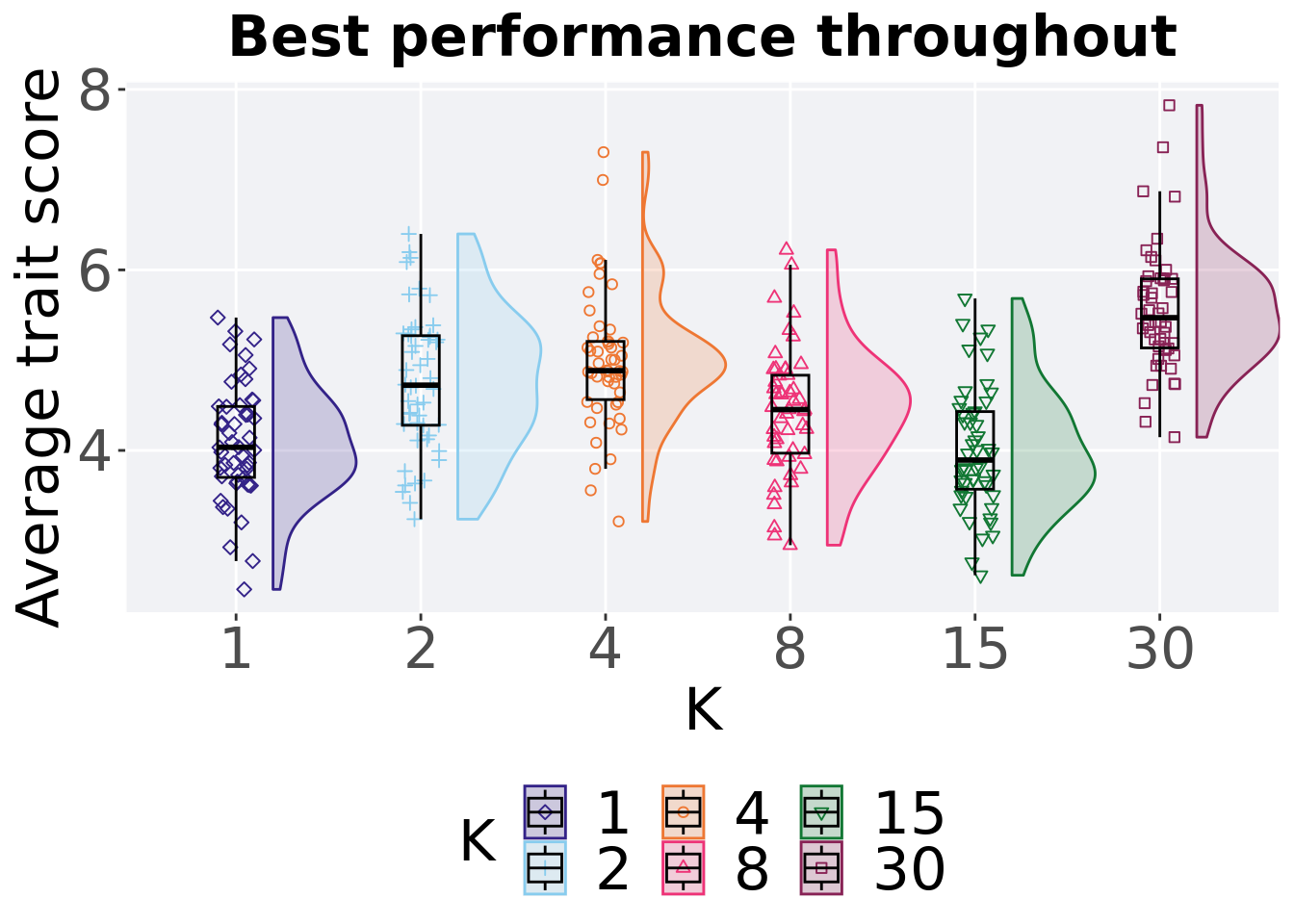
11.4.1.2.1 Stats
Summary statistics for the performance of the best performing solution found throughout 50,000 generations.
performance = filter(nov_best, col == 'pop_fit_max' & diagnostic == 'multipath_exploration')
group_by(performance, K) %>%
  dplyr::summarise(
    count = n(),
    na_cnt = sum(is.na(val)),
    min = min(val / DIMENSIONALITY, na.rm = TRUE),
    median = median(val / DIMENSIONALITY, na.rm = TRUE),
    mean = mean(val / DIMENSIONALITY, na.rm = TRUE),
    max = max(val / DIMENSIONALITY, na.rm = TRUE),
    IQR = IQR(val / DIMENSIONALITY, na.rm = TRUE)
  )
## # A tibble: 6 x 8
## K count na_cnt min median mean max IQR
## <fct> <int> <int> <dbl> <dbl> <dbl> <dbl> <dbl>
## 1 1 50 0 2.46 4.03 4.10 5.47 0.786
## 2 2 50 0 3.24 4.72 4.76 6.40 0.992
## 3 4 50 0 3.21 4.88 4.99 7.30 0.645
## 4 8 50 0 2.95 4.45 4.43 6.22 0.864
## 5 15 50 0 2.62 3.89 4.01 5.68 0.860
## 6 30 50 0 4.15 5.47 5.55 7.82 0.765Kruskal–Wallis test provides evidence of statistical differences among the best performing solution found throughout 50,000 generations.
##
##  Kruskal-Wallis rank sum test
##
## data:  val by K
## Kruskal-Wallis chi-squared = 112.24, df = 5, p-value < 2.2e-16
Results for post-hoc Wilcoxon rank-sum test with a Bonferroni correction on the best performing solution found throughout 50,000 generations.
pairwise.wilcox.test(x = performance$val, g = performance$K , p.adjust.method = "bonferroni",
                     paired = FALSE, conf.int = FALSE, alternative = 't')
##
## Pairwise comparisons using Wilcoxon rank sum test with continuity correction
##
## data: performance$val and performance$K
##
## 1 2 4 8 15
## 2 0.00070 - - - -
## 4 3.9e-07 1.00000 - - -
## 8 0.21797 0.45226 0.00187 - -
## 15 1.00000 0.00013 1.3e-07 0.03587 -
## 30 2.5e-13 2.8e-05 0.00061 4.2e-10 3.4e-13
##
## P value adjustment method: bonferroni11.4.1.3 End of 50,000 generations
Best performance in the population at the end of 50,000 generations.
filter(nov_ot, diagnostic == 'multipath_exploration' & gen == 50000) %>%
ggplot(., aes(x = K, y = pop_fit_max / DIMENSIONALITY, color = K, fill = K, shape = K)) +
  geom_flat_violin(position = position_nudge(x = .2, y = 0), scale = 'width', alpha = 0.2) +
  geom_point(position = position_jitter(width = .1), size = 1.5, alpha = 1.0) +
  geom_boxplot(color = 'black', width = .2, outlier.shape = NA, alpha = 0.0) +
  scale_y_continuous(
    name="Average trait score"
  ) +
  scale_x_discrete(
    name="K"
  )+
  scale_shape_manual(values=SHAPE)+
  scale_colour_manual(values = cb_palette) +
  scale_fill_manual(values = cb_palette) +
  ggtitle("Final performance") +
  p_theme
11.4.1.3.1 Stats
Summary statistics for the best performance in the population at the end of 50,000 generations.
performance = filter(nov_ot, diagnostic == 'multipath_exploration' & gen == 50000)
group_by(performance, K) %>%
  dplyr::summarise(
    count = n(),
    na_cnt = sum(is.na(pop_fit_max / DIMENSIONALITY)),
    min = min(pop_fit_max / DIMENSIONALITY, na.rm = TRUE),
    median = median(pop_fit_max / DIMENSIONALITY, na.rm = TRUE),
    mean = mean(pop_fit_max / DIMENSIONALITY, na.rm = TRUE),
    max = max(pop_fit_max / DIMENSIONALITY, na.rm = TRUE),
    IQR = IQR(pop_fit_max / DIMENSIONALITY, na.rm = TRUE)
  )
## # A tibble: 6 x 8
## K count na_cnt min median mean max IQR
## <fct> <int> <int> <dbl> <dbl> <dbl> <dbl> <dbl>
## 1 1 50 0 2.26 3.83 3.93 5.45 0.832
## 2 2 50 0 2.72 4.48 4.51 6.27 0.910
## 3 4 50 0 2.91 4.65 4.76 7.09 0.627
## 4 8 50 0 2.45 3.96 4.08 5.81 0.777
## 5 15 50 0 2.16 3.66 3.64 5.12 0.859
## 6 30 50 0 3.87 5.14 5.10 7.27 1.08Kruskal–Wallis test provides evidence of statistical differences among best performance in the population at the end of 50,000 generations.
##
##  Kruskal-Wallis rank sum test
##
## data:  pop_fit_max by K
## Kruskal-Wallis chi-squared = 95.737, df = 5, p-value < 2.2e-16
Results for post-hoc Wilcoxon rank-sum test with a Bonferroni correction on the best performance in the population at the end of 50,000 generations.
pairwise.wilcox.test(x = performance$pop_fit_max, g = performance$K , p.adjust.method = "bonferroni",
                     paired = FALSE, conf.int = FALSE, alternative = 't')
##
## Pairwise comparisons using Wilcoxon rank sum test with continuity correction
##
## data: performance$pop_fit_max and performance$K
##
## 1 2 4 8 15
## 2 0.01055 - - - -
## 4 4.1e-06 1.00000 - - -
## 8 1.00000 0.16610 0.00013 - -
## 15 0.63500 1.5e-05 5.2e-09 0.05030 -
## 30 2.3e-09 0.01195 0.38606 1.5e-07 4.0e-12
##
## P value adjustment method: bonferroni11.4.2 Activation gene coverage
Here we analyze the activation gene coverage for each parameter replicate on the multi-path exploration diagnostic.
11.4.2.1 Coverage over time
Activation gene coverage over time.
lines = filter(nov_ot, diagnostic == 'multipath_exploration') %>%
        group_by(K, gen) %>%
          dplyr::summarise(
            min = min(uni_str_pos),
            mean = mean(uni_str_pos),
            max = max(uni_str_pos)
          )
## `summarise()` has grouped output by 'K'. You can override using the `.groups`
## argument.ggplot(lines, aes(x=gen, y=mean, group = K, fill =K, color = K, shape = K)) +
geom_ribbon(aes(ymin = min, ymax = max), alpha = 0.1) +
geom_line(size = 0.5) +
geom_point(data = filter(lines, gen %% 2000 == 0 & gen != 0), size = 1.5, stroke = 2.0, alpha = 1.0) +
scale_y_continuous(
name="Coverage",
limits=c(-1, 101),
breaks=seq(0,100, 20),
labels=c("0", "20", "40", "60", "80", "100")
) +
scale_x_continuous(
name="Generations",
limits=c(0, 50000),
breaks=c(0, 10000, 20000, 30000, 40000, 50000),
labels=c("0e+4", "1e+4", "2e+4", "3e+4", "4e+4", "5e+4")
) +
scale_shape_manual(values=SHAPE)+
scale_colour_manual(values = cb_palette) +
scale_fill_manual(values = cb_palette) +
ggtitle("Activation gene coverage over time") +
p_theme
11.4.2.2 End of 50,000 generations
Activation gene coverage in the population at the end of 50,000 generations.
filter(nov_ot, diagnostic == 'multipath_exploration' & gen == 50000) %>%
ggplot(., aes(x = K, y = uni_str_pos, color = K, fill = K, shape = K)) +
  geom_flat_violin(position = position_nudge(x = .2, y = 0), scale = 'width', alpha = 0.2) +
  geom_point(position = position_jitter(width = .1), size = 1.5, alpha = 1.0) +
  geom_boxplot(color = 'black', width = .2, outlier.shape = NA, alpha = 0.0) +
  scale_y_continuous(
    name="Coverage"
  ) +
  scale_x_discrete(
    name="K"
  )+
  scale_shape_manual(values=SHAPE)+
  scale_colour_manual(values = cb_palette) +
  scale_fill_manual(values = cb_palette) +
  ggtitle("Final activation gene coverage") +
  p_theme
11.4.2.2.1 Stats
Summary statistics for the activation gene coverage in the population at the end of 50,000 generations.
coverage = filter(nov_ot, diagnostic == 'multipath_exploration' & gen == 50000)
group_by(coverage, K) %>%
  dplyr::summarise(
    count = n(),
    na_cnt = sum(is.na(uni_str_pos)),
    min = min(uni_str_pos, na.rm = TRUE),
    median = median(uni_str_pos, na.rm = TRUE),
    mean = mean(uni_str_pos, na.rm = TRUE),
    max = max(uni_str_pos, na.rm = TRUE),
    IQR = IQR(uni_str_pos, na.rm = TRUE)
  )
## # A tibble: 6 x 8
## K count na_cnt min median mean max IQR
## <fct> <int> <int> <int> <dbl> <dbl> <int> <dbl>
## 1 1 50 0 44 69.5 68.4 85 11.8
## 2 2 50 0 48 74.5 74.6 89 13.8
## 3 4 50 0 69 87 86.1 96 7.75
## 4 8 50 0 72 89 88.2 96 5
## 5 15 50 0 68 85.5 84.9 95 6
## 6 30 50 0 58 71 69.9 89 8Kruskal–Wallis test provides evidence of statistical differences among activation gene coverage in the population at the end of 50,000 generations.
##
##  Kruskal-Wallis rank sum test
##
## data:  uni_str_pos by K
## Kruskal-Wallis chi-squared = 176.13, df = 5, p-value < 2.2e-16
Results for post-hoc Wilcoxon rank-sum test with a Bonferroni correction on the activation gene coverage in the population at the end of 50,000 generations.
pairwise.wilcox.test(x = coverage$uni_str_pos, g = coverage$K , p.adjust.method = "bonferroni",
                     paired = FALSE, conf.int = FALSE, alternative = 't')
##
## Pairwise comparisons using Wilcoxon rank sum test with continuity correction
##
## data: coverage$uni_str_pos and coverage$K
##
## 1 2 4 8 15
## 2 0.025 - - - -
## 4 9.0e-14 5.3e-08 - - -
## 8 1.3e-15 2.4e-11 0.880 - -
## 15 2.7e-13 8.4e-07 1.000 0.017 -
## 30 1.000 0.035 2.5e-14 1.5e-15 1.3e-13
##
## P value adjustment method: bonferroni11.4.3 Multi-valley crossing
11.4.3.1 Performance over time
lines =  filter(nov_ot_mvc, diagnostic == 'multipath_exploration') %>%
  group_by(K, gen) %>%
  dplyr::summarise(
    min = min(pop_fit_max),
    mean = mean(pop_fit_max),
    max = max(pop_fit_max)
  )
## `summarise()` has grouped output by 'K'. You can override using the `.groups`
## argument.ggplot(lines, aes(x=gen, y=mean / DIMENSIONALITY, group = K, fill = K, color = K, shape = K)) +
geom_ribbon(aes(ymin = min / DIMENSIONALITY, ymax = max / DIMENSIONALITY), alpha = 0.1) +
geom_line(size = 0.5) +
geom_point(data = filter(lines, gen %% 2000 == 0 & gen != 0), size = 1.5, stroke = 2.0, alpha = 1.0) +
scale_y_continuous(
name="Average trait score"
) +
scale_x_continuous(
name="Generations",
limits=c(0, 50000),
breaks=c(0, 10000, 20000, 30000, 40000, 50000),
labels=c("0e+4", "1e+4", "2e+4", "3e+4", "4e+4", "5e+4")
) +
scale_shape_manual(values=SHAPE)+
scale_colour_manual(values = cb_palette) +
scale_fill_manual(values = cb_palette) +
ggtitle("Best performance over time") +
p_theme
11.4.3.2 Performance comparisons
# 80% and final generation comparison
end = filter(nov_ot_mvc, diagnostic == 'multipath_exploration' & gen == 50000)
end$Generation <- factor(end$gen)

mid = filter(nov_ot_mvc, diagnostic == 'multipath_exploration' & gen == 40000)
mid$Generation <- factor(mid$gen)

mvc_p = ggplot(mid, aes(x = K, y=pop_fit_max / DIMENSIONALITY, group = K, shape = Generation)) +
  geom_point(col = mvc_col[1] , position = position_jitternudge(jitter.width = .03, nudge.x = -0.05), size = 2, alpha = 1.0) +
  geom_boxplot(position = position_nudge(x = -.15, y = 0), lwd = 0.7, col = mvc_col[1], fill = mvc_col[1], width = .1, outlier.shape = NA, alpha = 0.0) +

  geom_point(data = end, aes(x = K, y=pop_fit_max / DIMENSIONALITY), col = mvc_col[2], position = position_jitternudge(jitter.width = .03, nudge.x = 0.05), size = 2, alpha = 1.0) +
  geom_boxplot(data = end, aes(x = K, y=pop_fit_max / DIMENSIONALITY), position = position_nudge(x = .15, y = 0), lwd = 0.7, col = mvc_col[2], fill = mvc_col[2], width = .1, outlier.shape = NA, alpha = 0.0) +

  scale_y_continuous(
    name="Average trait score"
  ) +
  scale_x_discrete(
    name="K"
  )+
  scale_shape_manual(values=c(0,1))+
  scale_colour_manual(values = c(mvc_col[1],mvc_col[2])) +
  p_theme

plot_grid(
  mvc_p +
    ggtitle("Performance comparisons") +
    theme(legend.position="none"),
  legend,
  nrow=2,
  rel_heights = c(1,.05),
  label_size = TSIZE
)
11.4.3.2.1 Stats
Summary statistics for the performance of the best performance at 40,000 and 50,000 generations.
# 80% and final generation comparison
slices = filter(nov_ot_mvc, diagnostic == 'multipath_exploration' & (gen == 50000 | gen == 40000))
slices$Generation <- factor(slices$gen, levels = c(50000,40000))
slices %>%
  group_by(K, Generation) %>%
  dplyr::summarise(
    count = n(),
    na_cnt = sum(is.na(pop_fit_max  / DIMENSIONALITY)),
    min = min(pop_fit_max  / DIMENSIONALITY, na.rm = TRUE),
    median = median(pop_fit_max  / DIMENSIONALITY, na.rm = TRUE),
    mean = mean(pop_fit_max  / DIMENSIONALITY, na.rm = TRUE),
    max = max(pop_fit_max  / DIMENSIONALITY, na.rm = TRUE),
    IQR = IQR(pop_fit_max  / DIMENSIONALITY, na.rm = TRUE)
  )
## `summarise()` has grouped output by 'K'. You can override using the `.groups`
## argument.## # A tibble: 12 x 9
## # Groups: K [6]
## K Generation count na_cnt min median mean max IQR
## <fct> <fct> <int> <int> <dbl> <dbl> <dbl> <dbl> <dbl>
## 1 1 50000 50 0 2.39 3.36 3.31 4.24 0.618
## 2 1 40000 50 0 1.93 2.94 2.94 4.19 0.603
## 3 2 50000 50 0 2.37 3.82 3.83 5.54 0.743
## 4 2 40000 50 0 1.99 3.42 3.42 4.64 0.590
## 5 4 50000 50 0 2.48 3.76 3.71 4.87 0.607
## 6 4 40000 50 0 2.18 3.31 3.33 4.26 0.609
## 7 8 50000 50 0 2.24 3.16 3.19 4.70 0.688
## 8 8 40000 50 0 2.10 2.94 2.92 4.36 0.611
## 9 15 50000 50 0 2.73 3.40 3.49 4.51 0.582
## 10 15 40000 50 0 2.42 3.11 3.10 3.87 0.538
## 11 30 50000 50 0 3.11 4.27 4.29 5.54 0.783
## 12 30 40000 50 0 2.29 3.77 3.80 4.98 0.662K 1
wilcox.test(x = filter(slices, K == 1 & Generation == 50000)$pop_fit_max,
            y = filter(slices, K == 1 & Generation == 40000)$pop_fit_max,
            alternative = 't')
##
## Wilcoxon rank sum test with continuity correction
##
## data: filter(slices, K == 1 & Generation == 50000)$pop_fit_max and filter(slices, K == 1 & Generation == 40000)$pop_fit_max
## W = 1808, p-value = 0.0001214
## alternative hypothesis: true location shift is not equal to 0K 2
wilcox.test(x = filter(slices, K == 2 & Generation == 50000)$pop_fit_max,
            y = filter(slices, K == 2 & Generation == 40000)$pop_fit_max,
            alternative = 't')
##
## Wilcoxon rank sum test with continuity correction
##
## data: filter(slices, K == 2 & Generation == 50000)$pop_fit_max and filter(slices, K == 2 & Generation == 40000)$pop_fit_max
## W = 1726, p-value = 0.001045
## alternative hypothesis: true location shift is not equal to 0K 4
wilcox.test(x = filter(slices, K == 4 & Generation == 50000)$pop_fit_max,
            y = filter(slices, K == 4 & Generation == 40000)$pop_fit_max,
            alternative = 't')
##
## Wilcoxon rank sum test with continuity correction
##
## data: filter(slices, K == 4 & Generation == 50000)$pop_fit_max and filter(slices, K == 4 & Generation == 40000)$pop_fit_max
## W = 1788, p-value = 0.000211
## alternative hypothesis: true location shift is not equal to 0K 8
wilcox.test(x = filter(slices, K == 8 & Generation == 50000)$pop_fit_max,
            y = filter(slices, K == 8 & Generation == 40000)$pop_fit_max,
            alternative = 't')
##
## Wilcoxon rank sum test with continuity correction
##
## data: filter(slices, K == 8 & Generation == 50000)$pop_fit_max and filter(slices, K == 8 & Generation == 40000)$pop_fit_max
## W = 1619, p-value = 0.01107
## alternative hypothesis: true location shift is not equal to 0K 15
wilcox.test(x = filter(slices, K == 15 & Generation == 50000)$pop_fit_max,
            y = filter(slices, K == 15 & Generation == 40000)$pop_fit_max,
            alternative = 't')
##
## Wilcoxon rank sum test with continuity correction
##
## data: filter(slices, K == 15 & Generation == 50000)$pop_fit_max and filter(slices, K == 15 & Generation == 40000)$pop_fit_max
## W = 1872, p-value = 1.831e-05
## alternative hypothesis: true location shift is not equal to 0K 30
wilcox.test(x = filter(slices, K == 30 & Generation == 50000)$pop_fit_max,
            y = filter(slices, K == 30 & Generation == 40000)$pop_fit_max,
            alternative = 't')
##
## Wilcoxon rank sum test with continuity correction
##
## data: filter(slices, K == 30 & Generation == 50000)$pop_fit_max and filter(slices, K == 30 & Generation == 40000)$pop_fit_max
## W = 1859, p-value = 2.73e-05
## alternative hypothesis: true location shift is not equal to 011.4.3.3 Activation gene coverage over time
lines = filter(nov_ot_mvc, diagnostic == 'multipath_exploration') %>%
  group_by(K, gen) %>%
  dplyr::summarise(
    min = min(uni_str_pos),
    mean = mean(uni_str_pos),
    max = max(uni_str_pos)
  )
## `summarise()` has grouped output by 'K'. You can override using the `.groups`
## argument.ggplot(lines, aes(x=gen, y=mean, group = K, fill =K, color = K, shape = K)) +
geom_ribbon(aes(ymin = min, ymax = max), alpha = 0.1) +
geom_line(size = 0.5) +
geom_point(data = filter(lines, gen %% 2000 == 0 & gen != 0), size = 1.5, stroke = 2.0, alpha = 1.0) +
scale_y_continuous(
name="Coverage"
) +
scale_x_continuous(
name="Generations",
limits=c(0, 50000),
breaks=c(0, 10000, 20000, 30000, 40000, 50000),
labels=c("0e+4", "1e+4", "2e+4", "3e+4", "4e+4", "5e+4")
) +
scale_shape_manual(values=SHAPE)+
scale_colour_manual(values = cb_palette) +
scale_fill_manual(values = cb_palette) +
ggtitle("Activation gene coverage over time") +
p_theme
11.4.3.4 Activation gene coverage comparison
Best performances in the population at 40,000 and 50,000 generations.
# 80% and final generation comparison
end = filter(nov_ot_mvc, diagnostic == 'multipath_exploration' & gen == 50000)
end$Generation <- factor(end$gen)

mid = filter(nov_ot_mvc, diagnostic == 'multipath_exploration' & gen == 40000)
mid$Generation <- factor(mid$gen)

mvc_p = ggplot(mid, aes(x = K, y=uni_str_pos, group = K, shape = Generation)) +
  geom_point(col = mvc_col[1] , position = position_jitternudge(jitter.width = .03, nudge.x = -0.05), size = 2, alpha = 1.0) +
  geom_boxplot(position = position_nudge(x = -.15, y = 0), lwd = 0.7, col = mvc_col[1], fill = mvc_col[1], width = .1, outlier.shape = NA, alpha = 0.0) +

  geom_point(data = end, aes(x = K, y=uni_str_pos), col = mvc_col[2], position = position_jitternudge(jitter.width = .03, nudge.x = 0.05), size = 2, alpha = 1.0) +
  geom_boxplot(data = end, aes(x = K, y=uni_str_pos), position = position_nudge(x = .15, y = 0), lwd = 0.7, col = mvc_col[2], fill = mvc_col[2], width = .1, outlier.shape = NA, alpha = 0.0) +

  scale_y_continuous(
    name="Coverage",
  ) +
  scale_x_discrete(
    name="K"
  )+
  scale_shape_manual(values=c(0,1))+
  scale_colour_manual(values = c(mvc_col[1],mvc_col[2])) +
  p_theme

plot_grid(
  mvc_p +
    ggtitle("Activation gene coverage over time") +
    theme(legend.position="none"),
  legend,
  nrow=2,
  rel_heights = c(1,.05),
  label_size = TSIZE
)
11.4.3.4.1 Stats
Summary statistics for the performance of the best performance at 40,000 and 50,000 generations.
slices = filter(nov_ot_mvc, diagnostic == 'multipath_exploration' & (gen == 50000 | gen == 40000))
slices$Generation <- factor(slices$gen, levels = c(50000,40000))
slices %>%
  group_by(K, Generation) %>%
  dplyr::summarise(
    count = n(),
    na_cnt = sum(is.na(uni_str_pos)),
    min = min(uni_str_pos, na.rm = TRUE),
    median = median(uni_str_pos, na.rm = TRUE),
    mean = mean(uni_str_pos, na.rm = TRUE),
    max = max(uni_str_pos, na.rm = TRUE),
    IQR = IQR(uni_str_pos, na.rm = TRUE)
  )
## `summarise()` has grouped output by 'K'. You can override using the `.groups`
## argument.## # A tibble: 12 x 9
## # Groups: K [6]
## K Generation count na_cnt min median mean max IQR
## <fct> <fct> <int> <int> <int> <dbl> <dbl> <int> <dbl>
## 1 1 50000 50 0 42 66 65.7 86 9.75
## 2 1 40000 50 0 42 66 65.6 86 9.75
## 3 2 50000 50 0 57 73 72.8 90 9.75
## 4 2 40000 50 0 57 73 72.7 90 9.75
## 5 4 50000 50 0 73 89 87.7 98 6.75
## 6 4 40000 50 0 72 89 87.5 98 6.75
## 7 8 50000 50 0 71 87 86.9 96 7.75
## 8 8 40000 50 0 69 87 86.5 95 7
## 9 15 50000 50 0 70 78 79.1 96 8.75
## 10 15 40000 50 0 66 77.5 78.6 96 8.75
## 11 30 50000 50 0 53 66 65.9 81 10
## 12 30 40000 50 0 52 65 65.0 81 10.5K 1
wilcox.test(x = filter(slices, K == 1 & Generation == 50000)$uni_str_pos,
            y = filter(slices, K == 1 & Generation == 40000)$uni_str_pos,
            alternative = 't')
##
## Wilcoxon rank sum test with continuity correction
##
## data: filter(slices, K == 1 & Generation == 50000)$uni_str_pos and filter(slices, K == 1 & Generation == 40000)$uni_str_pos
## W = 1262, p-value = 0.9367
## alternative hypothesis: true location shift is not equal to 0K 2
wilcox.test(x = filter(slices, K == 2 & Generation == 50000)$uni_str_pos,
            y = filter(slices, K == 2 & Generation == 40000)$uni_str_pos,
            alternative = 't')
##
## Wilcoxon rank sum test with continuity correction
##
## data: filter(slices, K == 2 & Generation == 50000)$uni_str_pos and filter(slices, K == 2 & Generation == 40000)$uni_str_pos
## W = 1257.5, p-value = 0.9614
## alternative hypothesis: true location shift is not equal to 0K 4
wilcox.test(x = filter(slices, K == 4 & Generation == 50000)$uni_str_pos,
            y = filter(slices, K == 4 & Generation == 40000)$uni_str_pos,
            alternative = 't')
##
## Wilcoxon rank sum test with continuity correction
##
## data: filter(slices, K == 4 & Generation == 50000)$uni_str_pos and filter(slices, K == 4 & Generation == 40000)$uni_str_pos
## W = 1287, p-value = 0.8007
## alternative hypothesis: true location shift is not equal to 0K 8
wilcox.test(x = filter(slices, K == 8 & Generation == 50000)$uni_str_pos,
            y = filter(slices, K == 8 & Generation == 40000)$uni_str_pos,
            alternative = 't')
##
## Wilcoxon rank sum test with continuity correction
##
## data: filter(slices, K == 8 & Generation == 50000)$uni_str_pos and filter(slices, K == 8 & Generation == 40000)$uni_str_pos
## W = 1304, p-value = 0.7115
## alternative hypothesis: true location shift is not equal to 0K 15
wilcox.test(x = filter(slices, K == 15 & Generation == 50000)$uni_str_pos,
            y = filter(slices, K == 15 & Generation == 40000)$uni_str_pos,
            alternative = 't')
##
## Wilcoxon rank sum test with continuity correction
##
## data: filter(slices, K == 15 & Generation == 50000)$uni_str_pos and filter(slices, K == 15 & Generation == 40000)$uni_str_pos
## W = 1295.5, p-value = 0.756
## alternative hypothesis: true location shift is not equal to 0K 30
wilcox.test(x = filter(slices, K == 30 & Generation == 50000)$uni_str_pos,
            y = filter(slices, K == 30 & Generation == 40000)$uni_str_pos,
            alternative = 't')
##
## Wilcoxon rank sum test with continuity correction
##
## data: filter(slices, K == 30 & Generation == 50000)$uni_str_pos and filter(slices, K == 30 & Generation == 40000)$uni_str_pos
## W = 1363.5, p-value = 0.4346
## alternative hypothesis: true location shift is not equal to 0