Chapter 6 Increasing population size versus increasing generations

6.1 Overview

# Relative location of data.
working_directory <-
  "experiments/2021-06-03-cardinality-pop-size/analysis/"
# working_directory <- "./"

# Settings for visualization
cb_palette <- "Set2"

# Create directory to dump plots
dir.create(paste0(working_directory, "imgs"), showWarnings=FALSE)

6.2 Analysis dependencies

library(ggplot2)
library(tidyverse)
library(knitr)
library(cowplot)
library(viridis)
library(RColorBrewer)
library(rstatix)
library(ggsignif)
library(Hmisc)
library(kableExtra)
source("https://gist.githubusercontent.com/benmarwick/2a1bb0133ff568cbe28d/raw/fb53bd97121f7f9ce947837ef1a4c65a73bffb3f/geom_flat_violin.R")

These analyses were conducted in the following computing environment:

print(version)

##                _                           
## platform       x86_64-pc-linux-gnu         
## arch           x86_64                      
## os             linux-gnu                   
## system         x86_64, linux-gnu           
## status                                     
## major          4                           
## minor          1.0                         
## year           2021                        
## month          05                          
## day            18                          
## svn rev        80317                       
## language       R                           
## version.string R version 4.1.0 (2021-05-18)
## nickname       Camp Pontanezen

6.3 Setup

data_loc <- paste0(working_directory, "data/timeseries.csv")
data <- read.csv(data_loc, na.strings="NONE")

data$cardinality <- as.factor(
  data$OBJECTIVE_CNT
)
data$selection_name <- as.factor(
  data$selection_name
)

data$epsilon <- as.factor(
  data$LEX_EPS
)

data$POP_SIZE <- as.factor(
  data$POP_SIZE
)

data <- filter(data, cardinality=="100") # These runs finished.
data$elite_trait_avg <-
  data$ele_agg_per / data$OBJECTIVE_CNT
data$unique_start_positions_coverage <-
  data$uni_str_pos / data$OBJECTIVE_CNT

final_data <- filter(data, evaluations==max(data$evaluations))

# Labeler for stats annotations
p_label <- function(p_value) {
  threshold = 0.0001
  if (p_value < threshold) {
    return(paste0("p < ", threshold))
  } else {
    return(paste0("p = ", p_value))
  }
}

# Significance threshold
alpha <- 0.05

####### misc #######
# Configure our default graphing theme
theme_set(theme_cowplot())

6.4 Exploration diagnostic performance

elite_ave_performance_fig <-
  ggplot(
    data,
    aes(
      x=evaluations,
      y=elite_trait_avg,
      color=POP_SIZE,
      fill=POP_SIZE
    )
  ) +
  stat_summary(geom="line", fun=mean) +
  stat_summary(
    geom="ribbon",
    fun.data="mean_cl_boot",
    fun.args=list(conf.int=0.95),
    alpha=0.2,
    linetype=0
  ) +
  scale_y_continuous(
    name="Average trait performance"
  ) +
  scale_x_continuous(
    name="Evaluations"
  ) +
  scale_fill_brewer(
    name="Population Size",
    palette=cb_palette
  ) +
  scale_color_brewer(
    name="Population Size",
    palette=cb_palette
  )
elite_ave_performance_fig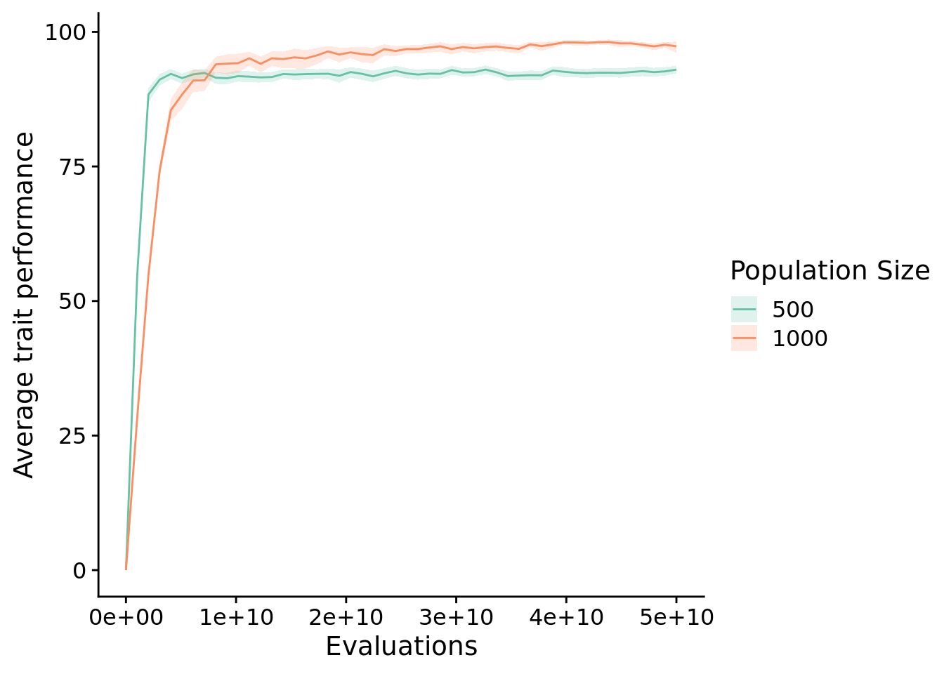

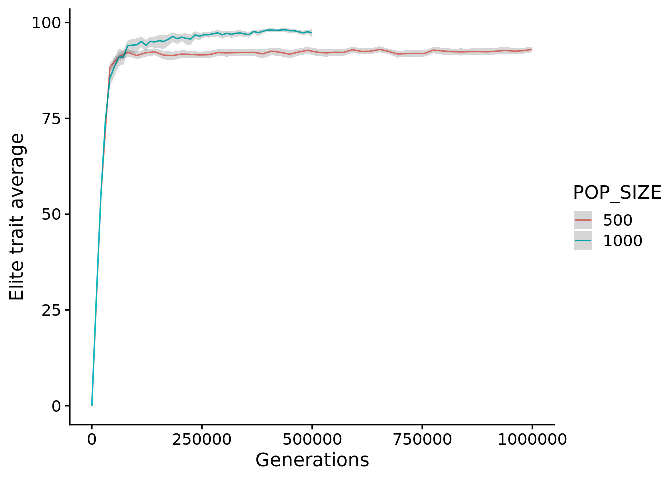
Same as above, but by generations instead of evaluations.

ggplot(data, aes(x=gen, y=elite_trait_avg, color=POP_SIZE)) +
  stat_summary(geom="line", fun=mean) +
  stat_summary(
    geom="ribbon",
    fun.data="mean_cl_boot",
    fun.args=list(conf.int=0.95),
    alpha=0.2,
    linetype=0
  ) +
  scale_y_continuous(
    name="Elite trait average"
  ) +
  scale_x_continuous(
    name="Generations"
  )

6.4.1 Final performance

# Compute manual labels for geom_signif
stat.test <- final_data %>%
  wilcox_test(elite_trait_avg ~ POP_SIZE) %>%
  adjust_pvalue(method = "bonferroni") %>%
  add_significance() %>%
  add_xy_position(x="POP_SIZE",step.increase=1)
stat.test$manual_position <- stat.test$y.position * 1.05
stat.test$label <- mapply(p_label,stat.test$p.adj)

elite_final_performance_fig <- ggplot(
    final_data,
    aes(x=POP_SIZE, y=elite_trait_avg, fill=POP_SIZE)
  ) +
  geom_flat_violin(
    position = position_nudge(x = .2, y = 0),
    alpha = .8,
    scale="width"
  ) +
  geom_point(
    mapping=aes(color=POP_SIZE),
    position = position_jitter(width = .15),
    size = .5,
    alpha = 0.8
  ) +
  geom_boxplot(
    width = .1,
    outlier.shape = NA,
    alpha = 0.5
  ) +
  scale_y_continuous(
    name="Average trait performance",
    limits=c(0, 100)
  ) +
  scale_x_discrete(
    name="Population Size"
  ) +
  scale_fill_brewer(
    name="Population Size",
    palette=cb_palette
  ) +
  scale_color_brewer(
    name="Population Size",
    palette=cb_palette
  ) +
  theme(
    legend.position="none"
  )
elite_final_performance_fig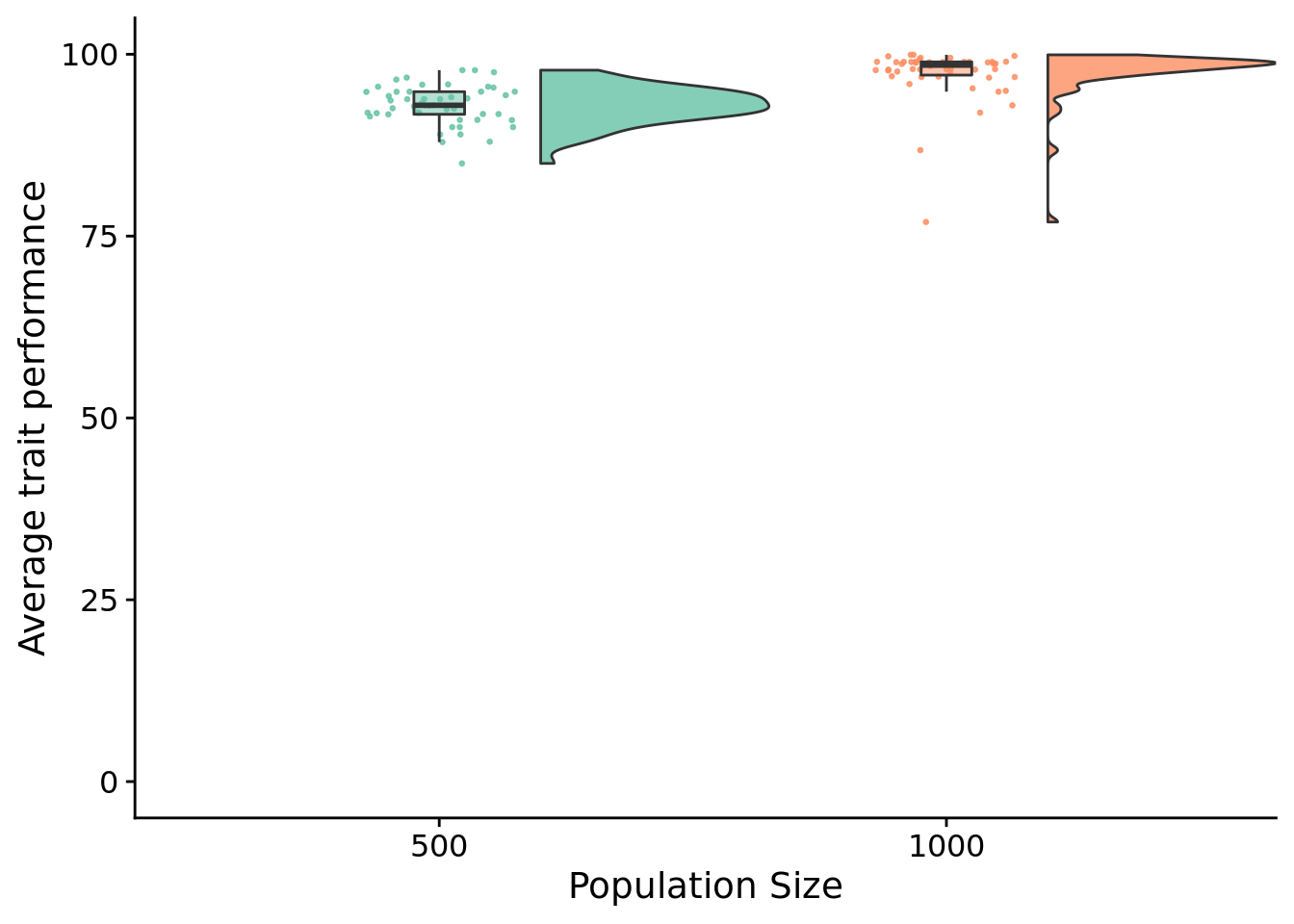

stat.test %>%
  kbl() %>%
  kable_styling(
    bootstrap_options = c(
      "striped",
      "hover",
      "condensed",
      "responsive"
    )
  ) %>%
  scroll_box(width="600px")

.y.	group1	group2	n1	n2	statistic	p	p.adj	p.adj.signif	y.position	groups	xmin	xmax	manual_position	label
elite_trait_avg	500	1000	50	50	219	0	0	****	102.036	500 , 1000	1	2	107.1378	p < 1e-04

6.5 Activation position coverage

unique_start_position_coverage_fig <- ggplot(
    data,
    aes(
      x=evaluations,
      y=unique_start_positions_coverage,
      color=POP_SIZE,
      fill=POP_SIZE
    )
  ) +
  stat_summary(geom="line", fun=mean) +
  stat_summary(
    geom="ribbon",
    fun.data="mean_cl_boot",
    fun.args=list(conf.int=0.95),
    alpha=0.2,
    linetype=0
  ) +
  scale_y_continuous(
    name="Activation position coverage",
    limits=c(0.0, 1.0)
  ) +
  scale_x_continuous(
    name="Evaluations"
  ) +
  scale_fill_brewer(
    name="Population Size",
    palette=cb_palette
  ) +
  scale_color_brewer(
    name="Population Size",
    palette=cb_palette
  )
unique_start_position_coverage_fig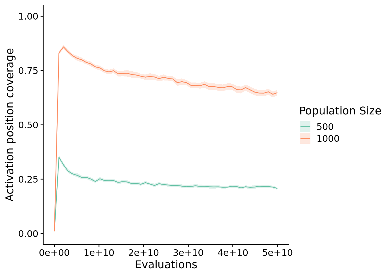

6.5.1 Final activation position coverage

# Compute manual labels for geom_signif
stat.test <- final_data %>%
  wilcox_test(unique_start_positions_coverage ~ POP_SIZE) %>%
  adjust_pvalue(method = "bonferroni") %>%
  add_significance() %>%
  add_xy_position(x="POP_SIZE",step.increase=1)
stat.test$manual_position <- stat.test$y.position * 1.05
stat.test$label <- mapply(p_label,stat.test$p.adj)

unique_start_positions_coverage_final_fig <- ggplot(
    final_data,
    aes(
      x=POP_SIZE,
      y=unique_start_positions_coverage,
      fill=POP_SIZE
    )
  ) +
  geom_flat_violin(
    position = position_nudge(x = .2, y = 0),
    alpha = .8,
    scale="width"
  ) +
  geom_point(
    mapping=aes(color=POP_SIZE),
    position = position_jitter(width = .15),
    size = .5,
    alpha = 0.8
  ) +
  geom_boxplot(
    width = .1,
    outlier.shape = NA,
    alpha = 0.5
  ) +
  scale_y_continuous(
    name="Activation position coverage",
    limits=c(0, 1.0)
  ) +
  scale_x_discrete(
    name="Population size"
  ) +
  scale_fill_brewer(
    name="Population size",
    palette=cb_palette
  ) +
  scale_color_brewer(
    name="Population size",
    palette=cb_palette
  ) +
  theme(
    legend.position="none"
  )
unique_start_positions_coverage_final_fig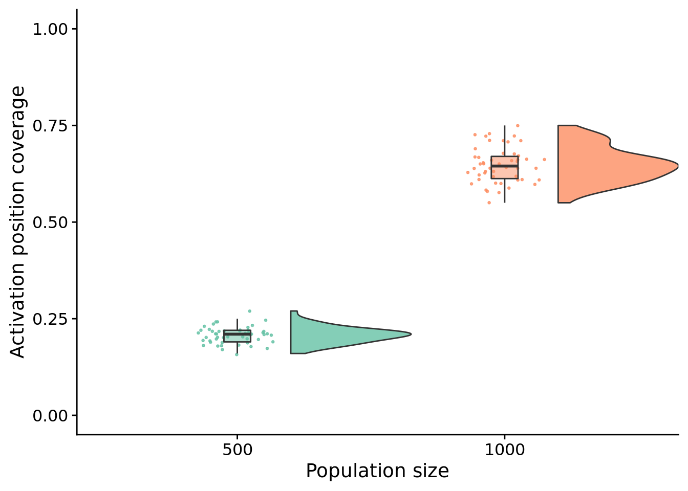

stat.test %>%
  kbl() %>%
  kable_styling(
    bootstrap_options = c(
      "striped",
      "hover",
      "condensed",
      "responsive"
    )
  ) %>%
  scroll_box(width="600px")

.y.	group1	group2	n1	n2	statistic	p	p.adj	p.adj.signif	y.position	groups	xmin	xmax	manual_position	label
unique_start_positions_coverage	500	1000	50	50	0	0	0	****	1.23	500 , 1000	1	2	1.2915	p < 1e-04

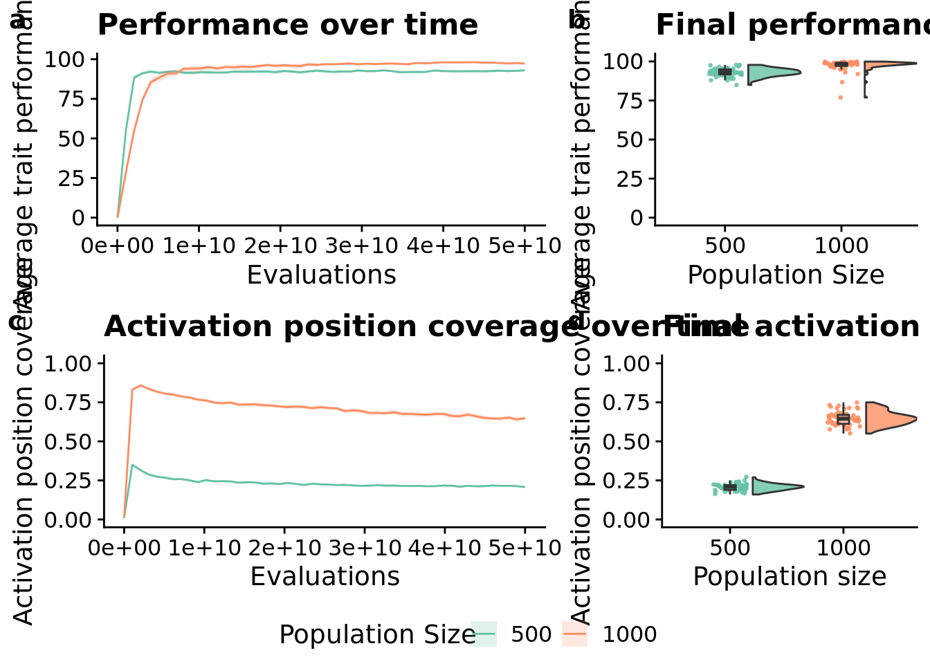
6.6 Manuscript figures

legend <- cowplot::get_legend(
    elite_ave_performance_fig +
      guides(
        color=guide_legend(nrow=1),
        fill=guide_legend(nrow=1)
      ) +
      theme(
        legend.position = "bottom",
        legend.box="horizontal",
        legend.justification="center"
      )
  )

grid <- plot_grid(
  elite_ave_performance_fig +
    ggtitle("Performance over time") +
    theme(legend.position="none"),
  elite_final_performance_fig +
    ggtitle("Final performance") +
    theme(),
  unique_start_position_coverage_fig +
    ggtitle("Activation position coverage over time") +
    theme(legend.position="none"),
  unique_start_positions_coverage_final_fig +
    ggtitle("Final activation position coverage") +
    theme(),
  nrow=2,
  ncol=2,
  rel_widths=c(3,2),
  labels="auto"
)

grid <- plot_grid(
  grid,
  legend,
  nrow=2,
  ncol=1,
  rel_heights=c(1, 0.1)
)


save_plot(
  paste(working_directory, "imgs/pop-size-panel.pdf", sep=""),
  grid,
  base_width=12,
  base_height=8
)

grid