Chapter 3 Ordered exploitation results
Here we present the results for best performances found by each selection scheme on the ordered exploitation diagnostic. 50 replicates are conducted for each scheme explored.
3.1 Data setup
DIR = paste(DATA_DIR,'ORDERED_EXPLOITATION/', sep = "", collapse = NULL)
over_time_df <- read.csv(paste(DIR,'over-time.csv', sep = "", collapse = NULL), header = TRUE, stringsAsFactors = FALSE)
over_time_df$scheme <- factor(over_time_df$scheme, levels = NAMES)

best_df <- read.csv(paste(DIR,'best.csv', sep = "", collapse = NULL), header = TRUE, stringsAsFactors = FALSE)
best_df$acro <- factor(best_df$acro, levels = ACRO)

sati_df <- read.csv(paste(DIR,'sol-fnd.csv', sep = "", collapse = NULL), header = TRUE, stringsAsFactors = FALSE)
sati_df$acro <- factor(sati_df$acro, levels = ACRO)
3.2 Performance over time
Best performance in a population over time. Data points on the graph is the average performance across 50 replicates every 2000 generations. Shading comes from the best and worse performance across 50 replicates.
lines = over_time_df %>%
  group_by(scheme, gen) %>%
  dplyr::summarise(
    min = min(pop_fit_max) / DIMENSIONALITY,
    mean = mean(pop_fit_max) / DIMENSIONALITY,
    max = max(pop_fit_max) / DIMENSIONALITY
  )
## `summarise()` has grouped output by 'scheme'. You can override using the
## `.groups` argument.lines$scheme <- factor(lines$scheme, levels = c('Truncation (tru)','Tournament (tor)','Lexicase (lex)','Random (ran)','Genotypic Fitness Sharing (gfs)','Phenotypic Fitness Sharing (pfs)','Nondominated Sorting (nds)','Novelty Search (nov)'))
over_time_plot = ggplot(lines, aes(x=gen, y=mean, group = scheme, fill = scheme, color = scheme, shape = scheme)) +
geom_ribbon(aes(ymin = min, ymax = max), alpha = 0.1) +
geom_line(size = 0.5) +
geom_point(data = filter(lines, gen %% 2000 == 0 & gen != 0), size = 1.5, stroke = 2.0, alpha = 1.0) +
scale_y_continuous(
name="Average trait score",
limits=c(0, 100),
breaks=seq(0,100, 20),
labels=c("0", "20", "40", "60", "80", "100")
) +
scale_x_continuous(
name="Generations",
limits=c(0, 50000),
breaks=c(0, 10000, 20000, 30000, 40000, 50000),
labels=c("0e+4", "1e+4", "2e+4", "3e+4", "4e+4", "5e+4")
) +
scale_shape_manual(values=c(5,3,1,20,2,6,0,4))+
scale_colour_manual(values = c('#332288','#88CCEE','#EE7733','#CCBB44','#EE3377','#117733','#882255','#44AA99')) +
scale_fill_manual(values = c('#332288','#88CCEE','#EE7733','#CCBB44','#EE3377','#117733','#882255','#44AA99')) +
ggtitle('Performance over time')+
p_theme +
guides(
shape=guide_legend(ncol=2, title.position = "left", title = 'Selection \nScheme'),
color=guide_legend(ncol=2, title.position = "left", title = 'Selection \nScheme'),
fill=guide_legend(ncol=2, title.position = "left", title = 'Selection \nScheme')
)
over_time_plot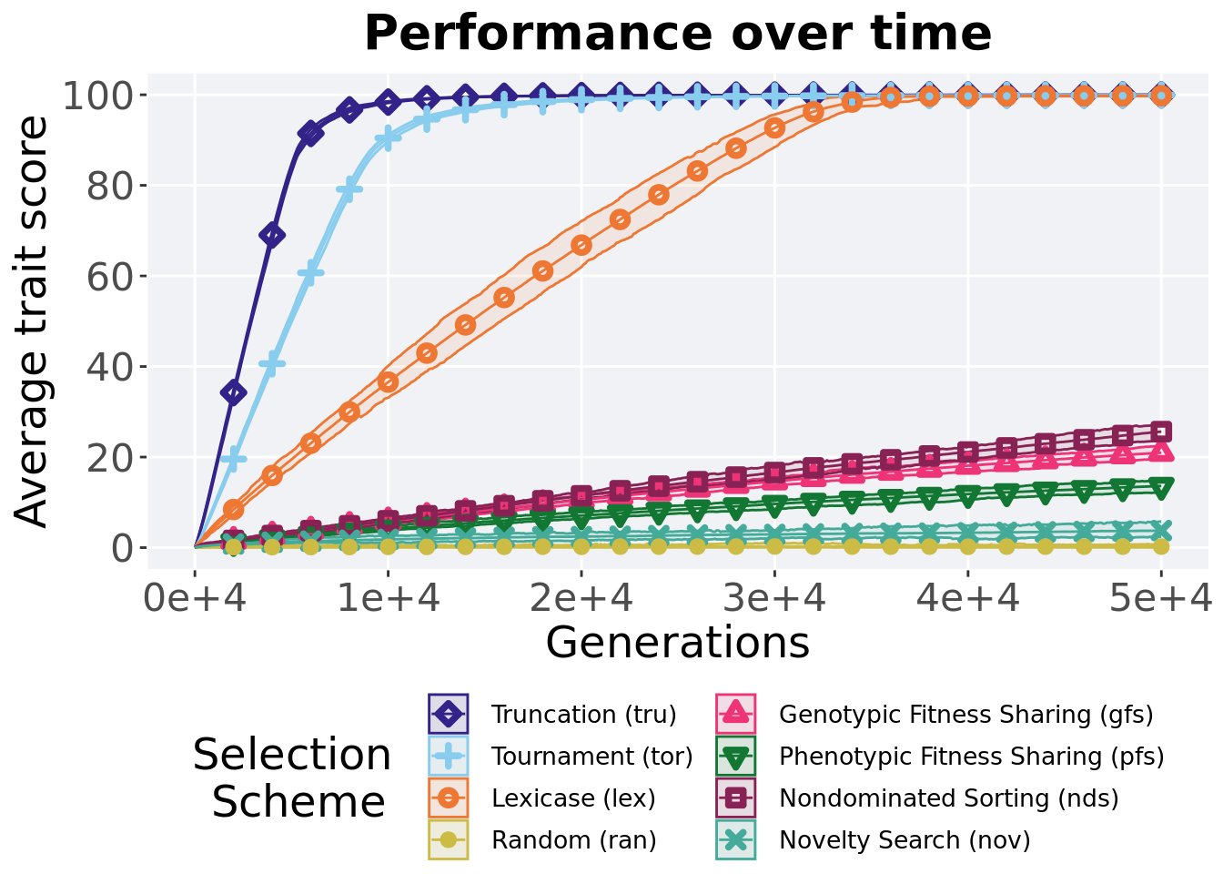
3.3 Best performance throughout
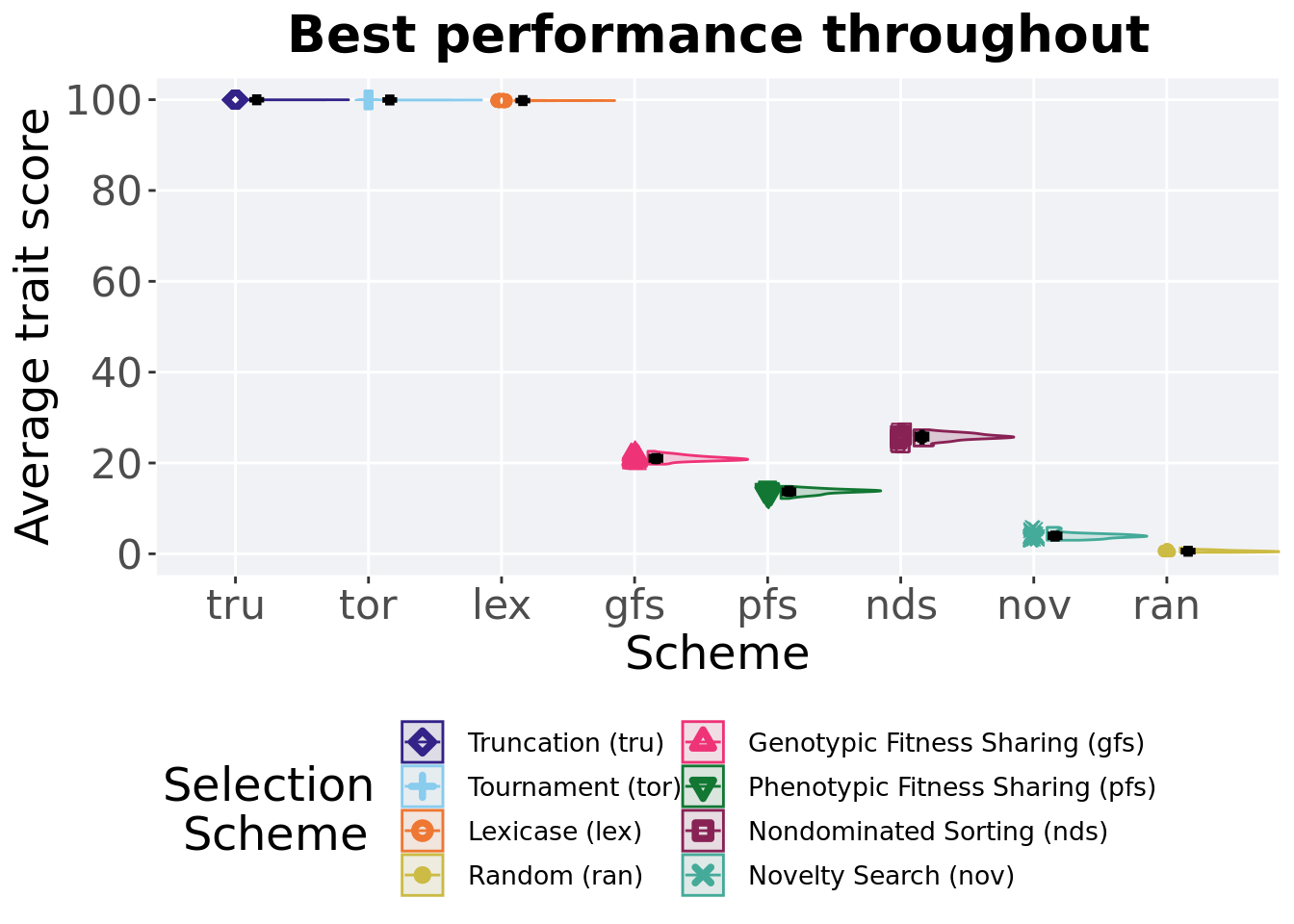
Best performance reached throughout 50,000 generations in a population.
plot = filter(best_df, var == 'pop_fit_max') %>%
  ggplot(., aes(x = acro, y = val / DIMENSIONALITY, color = acro, fill = acro, shape = acro)) +
  geom_flat_violin(position = position_nudge(x = .1, y = 0), scale = 'width', alpha = 0.2, width = 1.5) +
  geom_boxplot(color = 'black', width = .07, outlier.shape = NA, alpha = 0.0, size = 1.0, position = position_nudge(x = .16, y = 0)) +
  geom_point(position = position_jitter(width = 0.03, height = 0.02), size = 2.0, alpha = 1.0) +
  scale_y_continuous(
    name="Average trait score",
    limits=c(0, 100),
    breaks=seq(0,100, 20),
    labels=c("0", "20", "40", "60", "80", "100")
  ) +
  scale_x_discrete(
    name="Scheme"
  )+
  scale_shape_manual(values=SHAPE)+
  scale_colour_manual(values = cb_palette, ) +
  scale_fill_manual(values = cb_palette) +
  ggtitle('Best performance throughout')+
  p_theme

plot_grid(
  plot +
    theme(legend.position="none"),
  legend,
  nrow=2,
  rel_heights = c(3,1)
)
3.3.1 Stats
Summary statistics for the best performance.
performance = filter(best_df, var == 'pop_fit_max')
performance$acro = factor(performance$acro, levels = c('tru','tor','lex','nds','gfs','pfs','nov','ran'))
performance %>%
  group_by(acro) %>%
  dplyr::summarise(
    count = n(),
    na_cnt = sum(is.na(val)),
    min = min(val / DIMENSIONALITY, na.rm = TRUE),
    median = median(val / DIMENSIONALITY, na.rm = TRUE),
    mean = mean(val / DIMENSIONALITY, na.rm = TRUE),
    max = max(val / DIMENSIONALITY, na.rm = TRUE),
    IQR = IQR(val / DIMENSIONALITY, na.rm = TRUE)
  )
## # A tibble: 8 x 8
## acro count na_cnt min median mean max IQR
## <fct> <int> <int> <dbl> <dbl> <dbl> <dbl> <dbl>
## 1 tru 50 0 100. 100. 100. 100. 0.00168
## 2 tor 50 0 99.9 99.9 99.9 99.9 0.00650
## 3 lex 50 0 99.7 99.8 99.8 99.9 0.0247
## 4 nds 50 0 23.7 25.7 25.7 27.3 0.972
## 5 gfs 50 0 19.7 21.0 21.0 22.6 0.754
## 6 pfs 50 0 12.2 13.8 13.7 14.9 0.712
## 7 nov 50 0 3.00 3.90 4.00 5.83 0.666
## 8 ran 50 0 0.318 0.569 0.605 1.31 0.279Kruskal–Wallis test illustrates evidence of statistical differences.
##
##  Kruskal-Wallis rank sum test
##
## data:  val by acro
## Kruskal-Wallis chi-squared = 392.77, df = 7, p-value < 2.2e-16
Results for post-hoc Wilcoxon rank-sum test with a Bonferroni correction.
pairwise.wilcox.test(x = performance$val, g = performance$acro, p.adjust.method = "bonferroni",
                     paired = FALSE, conf.int = FALSE, alternative = 'l')
##
## Pairwise comparisons using Wilcoxon rank sum test with continuity correction
##
## data: performance$val and performance$acro
##
## tru tor lex nds gfs pfs nov
## tor <2e-16 - - - - - -
## lex <2e-16 <2e-16 - - - - -
## nds <2e-16 <2e-16 <2e-16 - - - -
## gfs <2e-16 <2e-16 <2e-16 <2e-16 - - -
## pfs <2e-16 <2e-16 <2e-16 <2e-16 <2e-16 - -
## nov <2e-16 <2e-16 <2e-16 <2e-16 <2e-16 <2e-16 -
## ran <2e-16 <2e-16 <2e-16 <2e-16 <2e-16 <2e-16 <2e-16
##
## P value adjustment method: bonferroni3.4 Generation satisfactory solution found
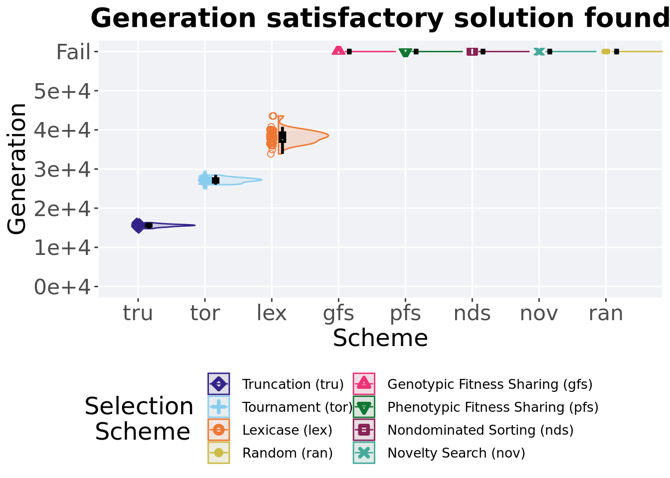
First generation a satisfactory solution is found throughout the 50,000 generations.
plot = sati_df %>%
  ggplot(., aes(x = acro, y = gen , color = acro, fill = acro, shape = acro)) +
  geom_flat_violin(position = position_nudge(x = .1, y = 0), scale = 'width', alpha = 0.2, width = 1.5) +
  geom_boxplot(color = 'black', width = .07, outlier.shape = NA, alpha = 0.0, size = 1.0, position = position_nudge(x = .16, y = 0)) +
  geom_point(position = position_jitter(width = 0.03, height = 0.02), size = 2.0, alpha = 1.0) +
  scale_y_continuous(
    name="Generation",
    limits=c(0, 60001),
    breaks=c(0, 10000, 20000, 30000, 40000, 50000, 60000),
    labels=c("0e+4", "1e+4", "2e+4", "3e+4", "4e+4", "5e+4", "Fail")
  ) +
  scale_x_discrete(
    name="Scheme"
  )+
  scale_shape_manual(values=SHAPE)+
  scale_colour_manual(values = cb_palette, ) +
  scale_fill_manual(values = cb_palette) +
  ggtitle('Generation satisfactory solution found')+
  p_theme

plot_grid(
  plot +
    theme(legend.position="none"),
  legend,
  nrow=2,
  rel_heights = c(3,1)
)
3.4.1 Stats
Summary statistics for the generation a satisfactory solution is found.
ssf = filter(sati_df, gen <= GENERATIONS)
ssf$acro = factor(ssf$acro, levels = c('tru','tor','lex'))
ssf %>%
  group_by(acro) %>%
  dplyr::summarise(
    count = n(),
    na_cnt = sum(is.na(gen)),
    min = min(gen, na.rm = TRUE),
    median = median(gen, na.rm = TRUE),
    mean = mean(gen, na.rm = TRUE),
    max = max(gen, na.rm = TRUE),
    IQR = IQR(gen, na.rm = TRUE)
  )
## # A tibble: 3 x 8
## acro count na_cnt min median mean max IQR
## <fct> <int> <int> <int> <dbl> <dbl> <int> <dbl>
## 1 tru 50 0 14776 15585 15570. 16317 420.
## 2 tor 50 0 25996 27138 27105. 28495 913.
## 3 lex 50 0 33877 38288. 38265. 43565 2215.Kruskal–Wallis test illustrates evidence of statistical differences.
##
##  Kruskal-Wallis rank sum test
##
## data:  gen by acro
## Kruskal-Wallis chi-squared = 132.45, df = 2, p-value < 2.2e-16
Results for post-hoc Wilcoxon rank-sum test with a Bonferroni correction.
pairwise.wilcox.test(x = ssf$gen, g = ssf$acro, p.adjust.method = "bonferroni",
                     paired = FALSE, conf.int = FALSE, alternative = 'g')
##
## Pairwise comparisons using Wilcoxon rank sum test with continuity correction
##
## data: ssf$gen and ssf$acro
##
## tru tor
## tor <2e-16 -
## lex <2e-16 <2e-16
##
## P value adjustment method: bonferroni3.5 Streaks over time
Longest streak of active geens for the best solution found in a population over time. A maximum streak value of 100 and a minimum streak value of 1 is possible. Data points on the graph is the average streak across 50 replicates every 2000 generations. Shading comes from the best and worse streak across 50 replicates.
lines = filter(over_time_df, acro != 'tor' & acro != 'tru' & acro != 'lex') %>%
  group_by(scheme, gen) %>%
  dplyr::summarise(
    min = min(ele_stk_cnt),
    mean = mean(ele_stk_cnt),
    max = max(ele_stk_cnt)
  )
## `summarise()` has grouped output by 'scheme'. You can override using the
## `.groups` argument.over_time_plot = ggplot(lines, aes(x=gen, y=mean, group = scheme, fill = scheme, color = scheme, shape = scheme)) +
geom_ribbon(aes(ymin = min, ymax = max), alpha = 0.1) +
geom_line(size = 0.5) +
geom_point(data = filter(lines, gen %% 2000 == 0 & gen != 0), size = 1.5, stroke = 2.0, alpha = 1.0) +
scale_y_continuous(
name="Streak",
limits=c(0, 45),
breaks=seq(0,45, 15)
) +
scale_x_continuous(
name="Generations",
limits=c(0, 50000),
breaks=c(0, 10000, 20000, 30000, 40000, 50000),
labels=c("0e+4", "1e+4", "2e+4", "3e+4", "4e+4", "5e+4")
) +
scale_shape_manual(values=STK_SHAPE)+
scale_colour_manual(values = stk_cb_palette) +
scale_fill_manual(values = stk_cb_palette) +
ggtitle('Longest streak over time')+
p_theme +
guides(
shape=guide_legend(ncol=2, title.position = "left", title = 'Selection \nScheme'),
color=guide_legend(ncol=2, title.position = "left", title = 'Selection \nScheme'),
fill=guide_legend(ncol=2, title.position = "left", title = 'Selection \nScheme')
)
over_time_plot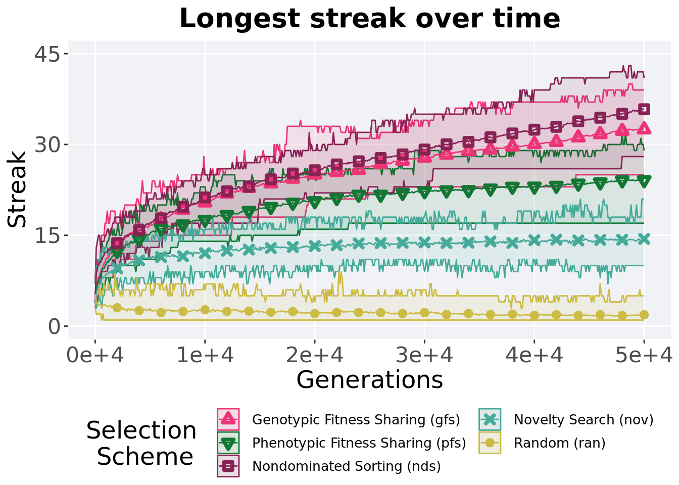
3.6 Longest streak throughout
Longest streak of the best solution found in the population throughout 50,000 generations.
plot = filter(best_df, var == 'ele_stk_cnt' &  acro != 'tor' & acro != 'tru' & acro != 'lex') %>%
  ggplot(., aes(x = acro, y = val, color = acro, fill = acro, shape = acro)) +
  geom_flat_violin(position = position_nudge(x = .1, y = 0), scale = 'width', alpha = 0.2, width = 1.5) +
  geom_boxplot(color = 'black', width = .07, outlier.shape = NA, alpha = 0.0, size = 1.0, position = position_nudge(x = .16, y = 0)) +
  geom_point(position = position_jitter(width = 0.03, height = 0.02), size = 2.0, alpha = 1.0) +
  scale_y_continuous(
    name="Streak",
    limits=c(0, 45),
    breaks=seq(0,45, 15)
  ) +
  scale_x_discrete(
    name="Scheme"
  )+
  scale_shape_manual(values=STK_SHAPE)+
  scale_colour_manual(values = stk_cb_palette) +
  scale_fill_manual(values = stk_cb_palette) +
  ggtitle('Longest streak throughout')+
  p_theme

plot_grid(
  plot +
    theme(legend.position="none"),
  legend,
  nrow=2,
  rel_heights = c(3,1)
)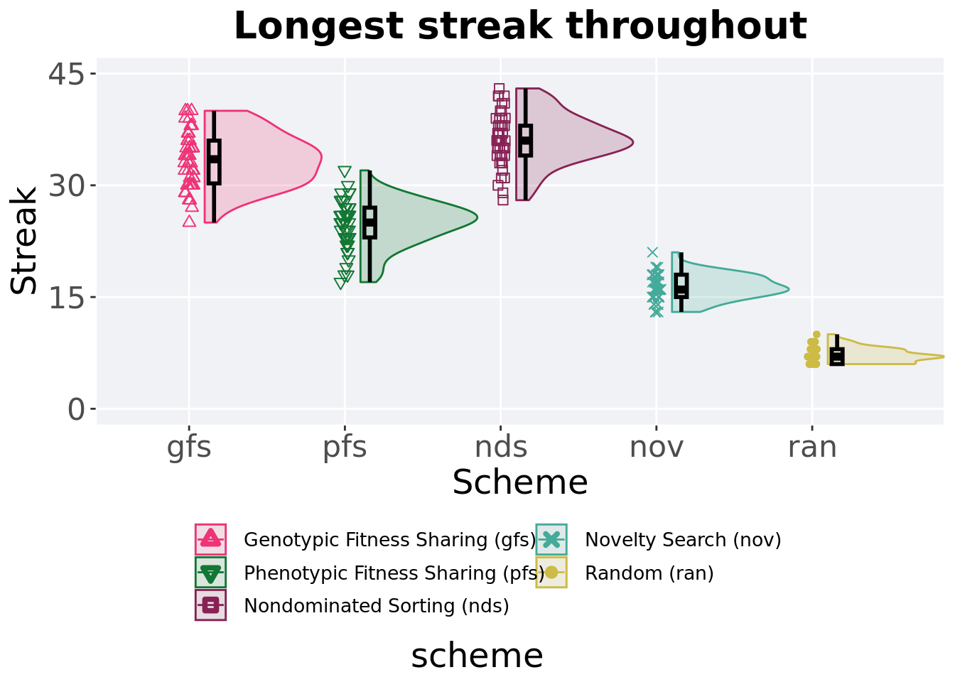
3.6.1 Stats
Summary statistics for the longest streak
streak = filter(best_df, var == 'ele_stk_cnt' &  acro != 'tor' & acro != 'tru' & acro != 'lex')
streak$acro = factor(streak$acro, levels = c('nds','gfs','pfs','nov','ran'))
streak %>%
  group_by(acro) %>%
  dplyr::summarise(
    count = n(),
    na_cnt = sum(is.na(val)),
    min = min(val, na.rm = TRUE),
    median = median(val, na.rm = TRUE),
    mean = mean(val, na.rm = TRUE),
    max = max(val, na.rm = TRUE),
    IQR = IQR(val, na.rm = TRUE)
  )
## # A tibble: 5 x 8
## acro count na_cnt min median mean max IQR
## <fct> <int> <int> <dbl> <dbl> <dbl> <dbl> <dbl>
## 1 nds 50 0 28 36 36.2 43 4
## 2 gfs 50 0 25 33.5 33.4 40 5.75
## 3 pfs 50 0 17 25 24.8 32 4
## 4 nov 50 0 13 16 16.3 21 3
## 5 ran 50 0 6 7 7.18 10 2Kruskal–Wallis test illustrates evidence of statistical differences.
##
##  Kruskal-Wallis rank sum test
##
## data:  val by acro
## Kruskal-Wallis chi-squared = 226.43, df = 4, p-value < 2.2e-16
Results for post-hoc Wilcoxon rank-sum test with a Bonferroni correction.
pairwise.wilcox.test(x = streak$val, g = streak$acro, p.adjust.method = "bonferroni",
                     paired = FALSE, conf.int = FALSE, alternative = 'l')
##
## Pairwise comparisons using Wilcoxon rank sum test with continuity correction
##
## data: streak$val and streak$acro
##
## nds gfs pfs nov
## gfs 0.0017 - - -
## pfs < 2e-16 2.7e-15 - -
## nov < 2e-16 < 2e-16 3.1e-16 -
## ran < 2e-16 < 2e-16 < 2e-16 < 2e-16
##
## P value adjustment method: bonferroni