Chapter 2 Nondominated sorting breakdown
For these experiments we break down nondominated sorting into its two main components: phenotypic fitness sharing and nondominated front ranking. We evaluated these components, along with standard nondominated sorting, on the contradictory objectives diagnostic to measure their contribution on the overall effectiveness of nondominated sorting. Here we present the results for activation gene coverage and satisfactory trait coverage found by each selection scheme on the contradictory objectives diagnostic. 50 replicates are conducted for each scheme explored.
2.2 Activation gene coverage over time
Activation gene coverage in a population over time. Data points on the graph is the average activation gene coverage across 50 replicates every 2000 generations. Shading comes from the best and worse coverage across 50 replicates.
lines = over_time_df %>%
  group_by(scheme, gen) %>%
  dplyr::summarise(
    min = min(uni_str_pos),
    mean = mean(uni_str_pos),
    max = max(uni_str_pos)
  )
## `summarise()` has grouped output by 'scheme'. You can override using the
## `.groups` argument.over_time_plot = ggplot(lines, aes(x=gen, y=mean, group = scheme, fill = scheme, color = scheme, shape = scheme)) +
geom_ribbon(aes(ymin = min, ymax = max), alpha = 0.1) +
geom_line(size = 0.5) +
geom_point(data = filter(lines, gen %% 2000 == 0 & gen != 0), size = 1.5, stroke = 2.0, alpha = 1.0) +
scale_y_continuous(
name="Coverage",
limits=c(0, 100),
breaks=seq(0,100, 20),
labels=c("0", "20", "40", "60", "80", "100")
) +
scale_x_continuous(
name="Generations",
limits=c(0, 50000),
breaks=c(0, 10000, 20000, 30000, 40000, 50000),
labels=c("0e+4", "1e+4", "2e+4", "3e+4", "4e+4", "5e+4")
) +
scale_shape_manual(values=SHAPE)+
scale_colour_manual(values = cb_palette) +
scale_fill_manual(values = cb_palette) +
ggtitle('Activation gene coverage over time')+
p_theme +
guides(
shape=guide_legend(ncol=1, title.position = "left", title = 'Selection \nScheme'),
color=guide_legend(ncol=1, title.position = "left", title = 'Selection \nScheme'),
fill=guide_legend(ncol=1, title.position = "left", title = 'Selection \nScheme')
)
over_time_plot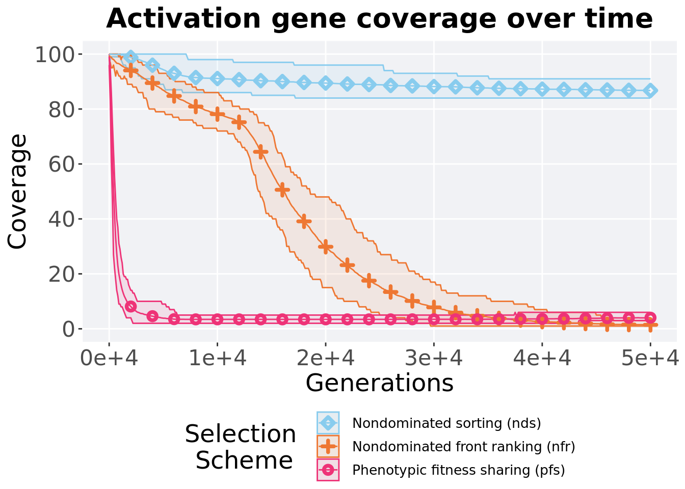
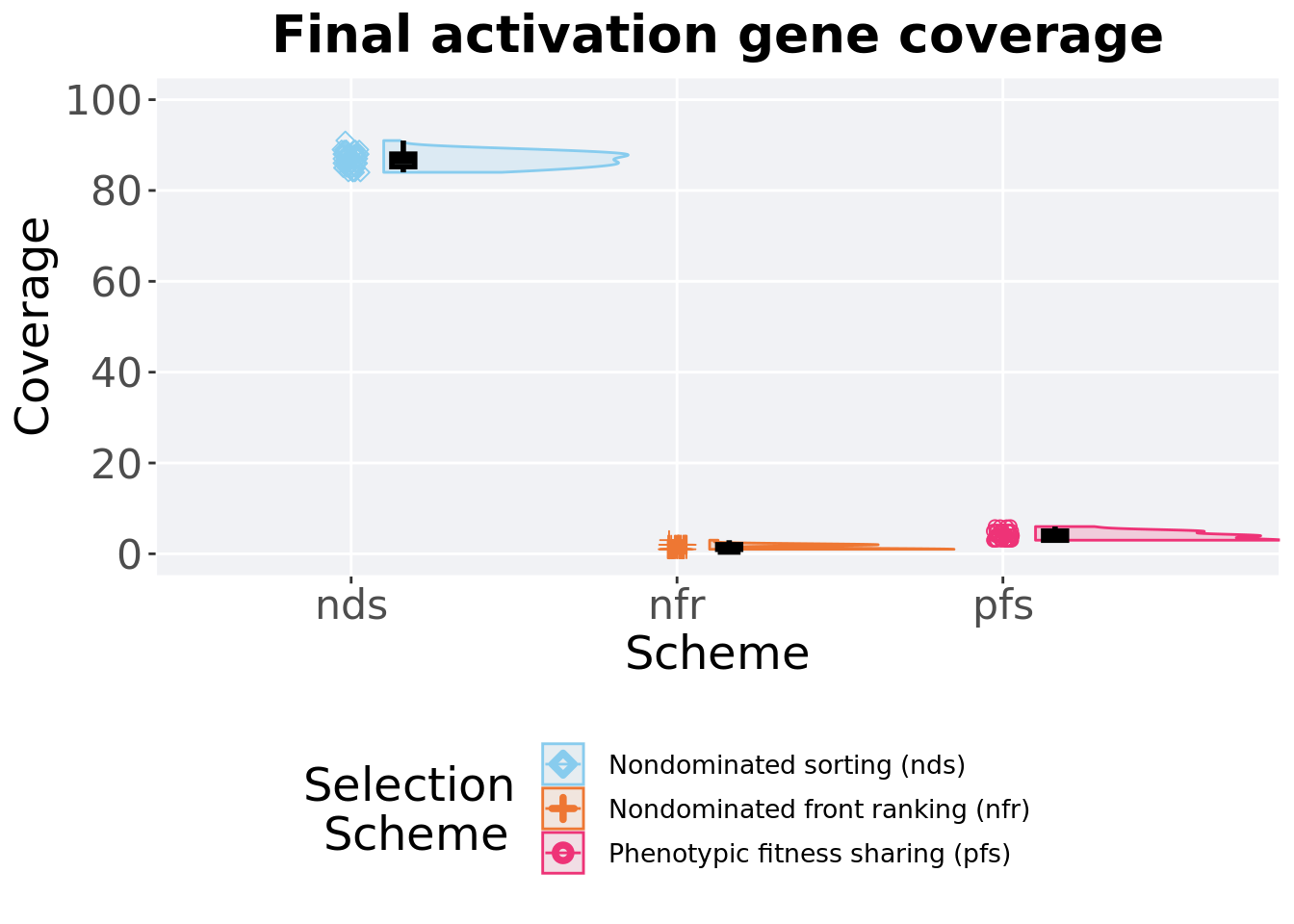
2.3 Final activation gene coverage
Activation gene coverage found in the final population at 50,000 generations.
plot = filter(over_time_df, gen == 50000) %>%
  ggplot(., aes(x = acro, y = uni_str_pos, color = acro, fill = acro, shape = acro)) +
  geom_flat_violin(position = position_nudge(x = .1, y = 0), scale = 'width', alpha = 0.2, width = 1.5) +
  geom_boxplot(color = 'black', width = .07, outlier.shape = NA, alpha = 0.0, size = 1.0, position = position_nudge(x = .16, y = 0)) +
  geom_point(position = position_jitter(width = 0.03, height = 0.02), size = 2.0, alpha = 1.0) +
  scale_y_continuous(
    name="Coverage",
    limits=c(0, 100),
    breaks=seq(0,100, 20),
    labels=c("0", "20", "40", "60", "80", "100")
  ) +
  scale_x_discrete(
    name="Scheme"
  )+
  scale_shape_manual(values=SHAPE)+
  scale_colour_manual(values = cb_palette, ) +
  scale_fill_manual(values = cb_palette) +
  ggtitle('Final activation gene coverage')+
  p_theme

plot_grid(
  plot +
    theme(legend.position="none"),
  legend,
  nrow=2,
  rel_heights = c(3,1)
)
2.3.1 Stats
Summary statistics for the coverage found in the final population.
act_coverage = filter(over_time_df, gen == 50000)
act_coverage$acro = factor(act_coverage$acro, levels = c('nds','pfs','nfr'))
act_coverage %>%
  group_by(acro) %>%
  dplyr::summarise(
    count = n(),
    na_cnt = sum(is.na(uni_str_pos)),
    min = min(uni_str_pos, na.rm = TRUE),
    median = median(uni_str_pos, na.rm = TRUE),
    mean = mean(uni_str_pos, na.rm = TRUE),
    max = max(uni_str_pos, na.rm = TRUE),
    IQR = IQR(uni_str_pos, na.rm = TRUE)
  )
## # A tibble: 3 x 8
## acro count na_cnt min median mean max IQR
## <fct> <int> <int> <int> <dbl> <dbl> <int> <dbl>
## 1 nds 50 0 84 87 86.8 91 2.75
## 2 pfs 50 0 3 4 4.04 6 2
## 3 nfr 50 0 1 1 1.44 3 1Kruskal–Wallis test illustrates evidence of statistical differences.
##
##  Kruskal-Wallis rank sum test
##
## data:  uni_str_pos by acro
## Kruskal-Wallis chi-squared = 133.91, df = 2, p-value < 2.2e-16
Results for post-hoc Wilcoxon rank-sum test with a Bonferroni correction.
pairwise.wilcox.test(x = act_coverage$uni_str_pos, g = act_coverage$acro, p.adjust.method = "bonferroni",
                     paired = FALSE, conf.int = FALSE, alternative = 'l')
##
## Pairwise comparisons using Wilcoxon rank sum test with continuity correction
##
## data: act_coverage$uni_str_pos and act_coverage$acro
##
## nds pfs
## pfs <2e-16 -
## nfr <2e-16 <2e-16
##
## P value adjustment method: bonferroni2.4 Satisfactory trait coverage over time
Satisfactory trait coverage in a population over time. Data points on the graph is the average activation gene coverage across 50 replicates every 2000 generations. Shading comes from the best and worse coverage across 50 replicates.
lines = over_time_df %>%
  group_by(scheme, gen) %>%
  dplyr::summarise(
    min = min(pop_uni_obj),
    mean = mean(pop_uni_obj),
    max = max(pop_uni_obj)
  )
## `summarise()` has grouped output by 'scheme'. You can override using the
## `.groups` argument.over_time_plot = ggplot(lines, aes(x=gen, y=mean, group = scheme, fill = scheme, color = scheme, shape = scheme)) +
geom_ribbon(aes(ymin = min, ymax = max), alpha = 0.1) +
geom_line(size = 0.5) +
geom_point(data = filter(lines, gen %% 2000 == 0 & gen != 0), size = 1.5, stroke = 2.0, alpha = 1.0) +
scale_y_continuous(
name="Coverage",
limits=c(0, 100),
breaks=seq(0,100, 20),
labels=c("0", "20", "40", "60", "80", "100")
) +
scale_x_continuous(
name="Generations",
limits=c(0, 50000),
breaks=c(0, 10000, 20000, 30000, 40000, 50000),
labels=c("0e+4", "1e+4", "2e+4", "3e+4", "4e+4", "5e+4")
) +
scale_shape_manual(values=SHAPE)+
scale_colour_manual(values = cb_palette) +
scale_fill_manual(values = cb_palette) +
ggtitle('Satisfactory trait coverage over time')+
p_theme +
guides(
shape=guide_legend(ncol=1, title.position = "left", title = 'Selection \nScheme'),
color=guide_legend(ncol=1, title.position = "left", title = 'Selection \nScheme'),
fill=guide_legend(ncol=1, title.position = "left", title = 'Selection \nScheme')
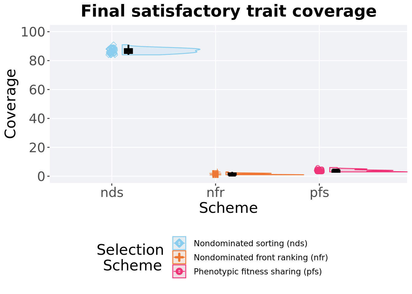
)2.5 Final satisfactory trait coverage
Satisfactory trait coverage found in the final population at 50,000 generations.
plot = filter(over_time_df, gen == 50000) %>%
  ggplot(., aes(x = acro, y = pop_uni_obj, color = acro, fill = acro, shape = acro)) +
  geom_flat_violin(position = position_nudge(x = .1, y = 0), scale = 'width', alpha = 0.2, width = 1.5) +
  geom_boxplot(color = 'black', width = .07, outlier.shape = NA, alpha = 0.0, size = 1.0, position = position_nudge(x = .16, y = 0)) +
  geom_point(position = position_jitter(width = 0.03, height = 0.02), size = 2.0, alpha = 1.0) +
  scale_y_continuous(
    name="Coverage",
    limits=c(0, 100),
    breaks=seq(0,100, 20),
    labels=c("0", "20", "40", "60", "80", "100")
  ) +
  scale_x_discrete(
    name="Scheme"
  )+
  scale_shape_manual(values=SHAPE)+
  scale_colour_manual(values = cb_palette, ) +
  scale_fill_manual(values = cb_palette) +
  ggtitle('Final satisfactory trait coverage')+
  p_theme

plot_grid(
  plot +
    theme(legend.position="none"),
  legend,
  nrow=2,
  rel_heights = c(3,1)
)
2.5.1 Stats
Summary statistics for the coverage found in the final population.
sat_coverage = filter(over_time_df, gen == 50000)
sat_coverage$acro = factor(sat_coverage$acro, levels = c('nds','pfs','nfr'))
sat_coverage %>%
  group_by(acro) %>%
  dplyr::summarise(
    count = n(),
    na_cnt = sum(is.na(pop_uni_obj)),
    min = min(pop_uni_obj, na.rm = TRUE),
    median = median(pop_uni_obj, na.rm = TRUE),
    mean = mean(pop_uni_obj, na.rm = TRUE),
    max = max(pop_uni_obj, na.rm = TRUE),
    IQR = IQR(pop_uni_obj, na.rm = TRUE)
  )
## # A tibble: 3 x 8
## acro count na_cnt min median mean max IQR
## <fct> <int> <int> <int> <dbl> <dbl> <int> <dbl>
## 1 nds 50 0 84 87 86.8 91 2.75
## 2 pfs 50 0 3 4 3.86 6 1
## 3 nfr 50 0 1 1 1.4 3 1Kruskal–Wallis test illustrates evidence of statistical differences.
##
##  Kruskal-Wallis rank sum test
##
## data:  pop_uni_obj by acro
## Kruskal-Wallis chi-squared = 134.12, df = 2, p-value < 2.2e-16
Results for post-hoc Wilcoxon rank-sum test with a Bonferroni correction.
pairwise.wilcox.test(x = sat_coverage$pop_uni_obj, g = sat_coverage$acro, p.adjust.method = "bonferroni",
                     paired = FALSE, conf.int = FALSE, alternative = 'l')
##
## Pairwise comparisons using Wilcoxon rank sum test with continuity correction
##
## data: sat_coverage$pop_uni_obj and sat_coverage$acro
##
## nds pfs
## pfs <2e-16 -
## nfr <2e-16 <2e-16
##
## P value adjustment method: bonferroni